A practical interview preparation repository for Machine Learning Engineer, AI Engineer, Data Scientist, Deep Learning Engineer, Data Engineer, and DevOps or platform-focused roles.
Please check out CrackingMachineLearningInterview GitPage(for Ui/UX experience).
Choose Your Track: answer one question about what you want to build, and get an ordered path through this repo for your role: ML Engineer, AI/GenAI Engineer, Data Scientist, Data Engineer, MLOps, or Deep Learning. Each track lists prerequisites, a stage-by-stage reading order, a project to build, and how to tell when you're interview-ready.
- Machine Learning Engineer
- Data Scientist
- Deep Learning Engineer
- AI Engineer
- Software Engineer working on AI/ML products
- Data Engineer
- MLOps Engineer
- DevOps / Platform Engineer
- New to the repo, or unsure where to begin? Start with Choose Your Track.
- Start with the 2026 Interview Roadmap if you are preparing for current AI/ML interviews.
- Use 2026 Additional Questions and Answers for modern interview rounds.
- Use the AI / GenAI, Data Engineering, and DevOps sections for specialized interview tracks.
- Use the Classic Question Bank for core ML, statistics, deep learning, and algorithms.
- Use Preparation Resources and References to build a targeted study plan.
- Use Suggested Learning Order if you want a clean path from fundamentals to production AI systems.
- The night before: skim the ML Cheat Sheet, drill the Glossary Flashcards, and rehearse a few Debugging Scenarios out loud.
- Choose Your Track: start here
- 2026 Interview Roadmap
- 2026 Additional Questions and Answers
- 2026 Common Interview Questions
- Behavioral & Project Deep-Dive Guide
- ML Take-Home Projects & Case Studies
- ML & AI Glossary
- ML Cheat Sheet: formulas & numbers for the night before
- ML Debugging Scenarios: "your model is broken, what do you do?"
- Glossary Flashcards: interactive practice
- AI / GenAI Track
- Classic ML Track
- Deep Learning Track
- MLOps Track
- Data Engineering Track
- DevOps Track
- Coding Challenges Track
- Cloud ML Platforms
- System Design Track
- Frameworks Track
- Project Setup & Engineering Track
- Suggested Learning Order
- Highlighted Projects
- Preparation Resources and References
- Study Pattern
- Classic Question Bank
- Contributions
- Github Profile: Shafaypro ©
- Repository: CrackingMachineLearningInterview
- Image references are included for educational purposes. Please see the repository references for attribution where applicable.
Feel free to share the repository link in your blog, study notes, or interview preparation material.
docs/choose-your-track.md: pick a track by goal or background, then follow a staged path through the repo for that role.docs/2026-interview-roadmap.md: current interview focus areas for ML Engineer and AI Engineer roles.docs/2026-additional-questions.md: modern 2026 question bank covering LLMs, RAG, evaluation, agents, and production AI.docs/interview_questions_2026.md: deep-dive interview Q&A covering agents, RAG, LLM scaling, production AI, and system design.docs/resources-and-references.md: books, references, and additional interview topics.docs/study-pattern.md: recommended preparation topics, difficulty levels, and study structure.docs/behavioral-interview-guide.md: STAR stories, the project deep-dive round, ML-specific behavioral questions, and level expectations.docs/take-home-projects.md: what reviewers score, time budgeting, repository structure, and the follow-up presentation round.docs/glossary.md: every term in the repo defined in a sentence or two, with the practical point attached.docs/ml-cheat-sheet.md: metrics, losses, distributions, update rules, and the numbers worth memorising, on one page.docs/ml-debugging-scenarios.md: troubleshooting scenarios (leakage, NaN loss, offline/online gaps, drift, RAG regressions) with ranked causes and fixes.flashcards.html: interactive flashcards built from the glossary, with progress saved in your browser.tools/check_links.py: offline link and anchor checker, run in CI on every pull request.ai_genai/: GenAI and LLM engineering topics including n8n, CrewAI, LangGraph, LangSmith, multi-agent systems, and advanced RAG.classical_ml/: classical ML algorithms and the math behind them, linear algebra and optimization, time series, clustering, dimensionality reduction, recommender systems, feature engineering.mlops/: MLOps topics, MLflow, model serving, feature stores, explainability, data quality, data labeling and active learning, responsible AI, LLM evaluation.cloud_ml/: cloud ML platforms, AWS SageMaker, Google Vertex AI, Azure ML.data_engineering/: data engineering interview topics, platform concepts, and geospatial AI.devops/: DevOps, infrastructure, deployment, and AI testing topics.frameworks/: ML and AI frameworks including FastAPI, Pydantic, PyTorch, HuggingFace, and LLM serving.system_design/: ML system design patterns, RAG pipelines, agent architectures, batch vs real-time systems.deep_learning/: deep learning fundamentals, transformers, applied training pipelines, distributed training, and reinforcement learning.coding_challenges/: Python and SQL interview practice guides for coding screens and data problem solving.project_setup/: how to set up a project on GitHub and structure real ML/AI/agent/data-engineering repositories.README.md: repository landing page plus the original classic ML interview question bank.
Use this order if you want to move from theory to production-grade AI engineering:
- Classic ML Track
- Deep Learning Track
- AI / GenAI Track
- Data Engineering Track
- MLOps Track
- Frameworks Track
- System Design Track
- Coding Challenges Track
- Cloud ML Platforms
- Project Setup & Engineering Track: ship it the right way
Use these to turn the repo into a portfolio, not just a reading list:
- Training and Inference Pipeline
- Prompt Experimentation Repo
- Multi-Agent Research Assistant
- Multi-Model Router
- Document Understanding System
- AI Workflow Automation with n8n
- Eval Pipeline
- CI/CD for AI App
- Scalable AI API
- Feature Store System
Use this track for AI Engineer, GenAI Engineer, LLM Engineer, Applied AI, and agent-platform interviews.
Core topics:
- The Agentic AI Engineer Roadmap (34-topic curriculum: foundation → frontier)
- LLM & Generative AI Fundamentals
- RAG
- RAG Engineering
- Context Engineering (budgets, ordering, caching, memory, compaction)
- Embeddings (models, chunking, fine-tuning, quantization)
- Vector Databases
- Vector Databases: Advanced (Pinecone, Weaviate, FAISS, pgvector, Hybrid Search, Reranking)
- LLM Inference Optimization (KV cache, batching, quantization, speculative decoding)
- LLMOps
- Agentic AI
- Agent Systems & Tool Use
- Multi-Agent Systems (Patterns, Memory, Tool Calling, Failure Handling)
- Multi-Model & AI Orchestration
- Multimodal AI
- CrewAI
- n8n - AI Workflow Automation
- n8n - Advanced AI Workflows
- LangGraph
- LangSmith: Observability & Evaluation
- Prompt Engineering (CoT, ReAct, Few-Shot, Self-Consistency, ToT, Output Control)
- Structured Outputs & Function Calling (JSON Mode, Tool Use, Pydantic, Instructor)
- LLM Security (Prompt Injection, Jailbreaks, Red-Teaming, Defenses)
- MCP
- LangChain
- Anthropic Overview
Use this track for pipeline, ETL, orchestration, warehouse, lakehouse, streaming, and geospatial interviews.
Core topics:
- Data Engineering for AI
- Data Modeling
- Data Architecture
- Types of Data Processing Pipelines (Batch → Streaming, When-to-Use-What)
- Apache Spark
- Apache Kafka
- Apache Airflow
- dbt Introduction
- dbt Interview Guide
- Apache Iceberg
- Delta Lake
- DuckDB
- OpenClaw (illustrative lineage example; see the note in the guide)
- Geospatial AI Systems (Google Solar API, ArcGIS, PostGIS, H3)
Use this track for ML engineer, deep learning engineer, and applied AI interviews requiring architecture and training depth.
Core topics:
- Deep Learning Overview
- Applied Deep Learning Roadmap
- Sequence Models (RNN, LSTM, GRU, Seq2Seq, Attention)
- Transformers
- Neural Network Training (optimizers, normalization, regularization, debugging)
- Generative Models (VAEs, GANs, Diffusion, Latent Diffusion)
- Graph Neural Networks (message passing, GCN, GraphSAGE, GAT)
- Model Compression (distillation, pruning, quantization)
- Distributed Training (DDP, FSDP/ZeRO, tensor & pipeline parallelism, mixed precision)
- Reinforcement Learning (MDPs, Q-learning, bandits, PPO, offline RL, RLHF)
- Speech & Audio ML (log-mel, CTC, RNN-T, Whisper, TTS, voice agents)
- Computer Vision (CNNs, Detection, Segmentation, ViT)
- Fine-Tuning (LoRA, QLoRA, PEFT, RLHF/DPO)
Use this track for infrastructure, CI/CD, containers, orchestration, IaC, and AI system testing interviews.
Core topics:
- Docker
- Kubernetes
- Helm
- Terraform
- GitHub Actions
- Observability (metrics, logs, traces, SLOs, Prometheus, OpenTelemetry)
- Testing AI Systems (Playwright, Puppeteer, LLM E2E Testing)
Use this track for classical ML algorithm interviews, data science roles, and as foundations for ML engineer roles.
Core topics:
- Math for ML (linear algebra, calculus, optimization, numerical stability)
- Model Evaluation & Metrics (ROC vs PR, calibration, thresholds, CV)
- Ensemble Methods & Gradient Boosting (RF, XGBoost, LightGBM, CatBoost)
- Causal Inference & Uplift Modeling (DiD, IV, RDD, CATE, Qini)
- Anomaly Detection (Isolation Forest, LOF, autoencoders, time series)
- NLP Fundamentals (tokenization, TF-IDF, embeddings, NER)
- Statistics & Probability
- Time Series & Forecasting
- Clustering Algorithms
- Dimensionality Reduction
- Recommender Systems
- Feature Engineering & Selection
Use this track for MLOps Engineer, Senior ML Engineer, and production ML system interviews.
Core topics:
- LLMOps / MLOps Engineering
- CI/CD for Machine Learning (registry, gates, canary, rollback)
- MLflow
- Model Explainability (SHAP, LIME)
- Feature Stores
- Model Serving
- Data Quality & Validation
- LLM Evaluation (Evals, Benchmarks, Hallucination Detection, HITL)
- Evaluation & Guardrails
- A/B Testing for ML (Experiment Design, Stats, Online Metrics)
- Data Labeling, Active Learning & Weak Supervision
- Responsible AI: Fairness, Bias, Privacy & Governance
Use this track for cloud-specific ML engineer and MLOps roles at companies using AWS, GCP, or Azure.
Core topics:
- Cloud ML Platforms Overview
- Cloud ML Platforms Comparison (SageMaker vs Vertex AI vs Azure ML)
- AWS SageMaker Interview Guide
- Google Vertex AI Interview Guide
- Azure Machine Learning Interview Guide
Use this track for senior ML engineer, staff engineer, and principal engineer interviews requiring system design depth.
Core topics:
- ML System Design Framework & Patterns
- Backend & System Design for AI
- Recommendation System Design
- Search & Ranking System Design
- Designing a Production LLM Assistant
- Fraud Detection System Design
- Ads Click-Through-Rate Prediction System Design (auctions, calibration, delayed feedback)
- Content Moderation System Design (multimodal, human review, prevalence)
- ETA Prediction System Design (routing baseline, residual models, quantile losses)
- News Feed Ranking System Design (value model, multi-task ranking, fan-out)
- Visual Search System Design (metric learning, ANN indexes, re-ranking)
- Enterprise RAG Search System Design (connectors, permissions, hybrid retrieval, evaluation)
- Notification Ranking System Design (send budgets, incrementality, send-time optimization)
- Dynamic Pricing System Design (causal elasticity, surge, switchback experiments)
- People You May Know System Design (link prediction, graph candidates, privacy)
- ML System Design Patterns: RAG, Agents, Batch vs Real-Time (2026)
Use this track for interview rounds that require live coding, take-home problem solving, or SQL assessments.
Core topics:
- Coding Challenges Overview
- Python Coding Challenges
- SQL Coding Challenges
- ML Coding Challenges: Implement From Scratch
- Pandas & NumPy Challenges
Use this track for roles requiring hands-on Python API development and AI framework expertise.
Core topics:
- Python for AI Engineering (async, type hints, Pydantic, APIs, logging)
- PyTorch
- HuggingFace
- LangChain
- Ollama
- vLLM
- Unsloth
- FastAPI: Production AI Backend Engineering
- Pydantic: Data Validation for AI Systems
Use this track to learn the engineering hygiene every ML/AI Engineer is expected to have: shipping projects on GitHub and structuring real repositories.
Core topics:
- Project Setup & Engineering Overview
- How to Set Up a Project on GitHub (Git, Branching, PRs, CI, Pages, Secrets)
- ML/AI Project Folder Structures (ML, DL, LLM, Agents, Data Eng)
    Supervised learning is when you know the outcome and you are provided with the fully labeled outcome data while in unsupervised you are not
    provided with labeled outcome data. Fully labeled means that each example in the training dataset is tagged with the answer the algorithm should
    come up with on its own. So, a labeled dataset of flower images would tell the model which photos were of roses, daisies and daffodils. When shown
    a new image, the model compares it to the training examples to predict the correct label.

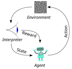
    A learning differs from supervised learning in not needing labelled input/output pairs be presented, and in not needing sub-optimal actions to be
    explicitly corrected. Instead the focus is on finding a balance between exploration (of uncharted territory) and exploitation (of current
    knowledge). In reinforcement learning each learning step involves a penalty criteria whether to give the model positive points or negative points
    and based on that penalizing the model.
    Deep learning is defined as algorithms inspired by the structure and function of the brain called artificial neural networks(ANN).Deep learning
    most probably focuses on Non Linear Analysis and is recommend for Non Linear problems regarding Artificial Intelligence.
    Deep learning is a subset of machine learning, and both are subsets of AI. The practical difference is where the features come from.

    Classical ML (linear models, trees, gradient boosting, SVMs) learns from features that people design: ratios, counts,
    TF-IDF vectors, aggregates. Deep learning stacks many layers of learned non-linear transformations, so the network
    learns its own features directly from raw inputs such as pixels, audio samples or tokens.

    Neither one "knows on its own" whether a prediction is correct. Both learn by minimising a loss against labels
    (or a self-supervised target) with an optimiser.

    Rules of thumb:
        * Tabular data, small or medium datasets, need for interpretability -> gradient boosting is usually the strong baseline.
        * Images, audio, text, video, very large datasets -> deep learning wins because hand-built features plateau.
        * Deep learning needs more data, more compute (GPUs) and more tuning, and is harder to explain.

    Semi-supervised learning uses a small amount of labeled data combined with a large amount of unlabeled data during training. It sits between
    supervised (fully labeled) and unsupervised (no labels) learning. Common techniques include self-training, label propagation, and generative
    models. Example: training an image classifier with 100 labeled images and 10,000 unlabeled ones.

    Reinforcement learning (RL) is a paradigm where an agent learns by interacting with an environment, receiving rewards or penalties based on its
    actions. Unlike semi-supervised learning which works on a fixed dataset, RL involves sequential decision making. The agent learns a policy that
    maximizes cumulative reward over time. Example: training a robot to walk or an agent to play chess.
    Bias is error from wrong or overly simple assumptions: the model cannot represent the true relationship, so it is
    wrong in the same way on every training set (underfitting). Example: a straight line fitted to a curve.

    Variance is error from sensitivity to the particular training sample: the model fits noise, so retraining on a
    different sample gives a very different model (overfitting). Example: a fully grown decision tree.

    For squared loss, expected test error = Bias^2 + Variance + irreducible noise.

    Reduce bias: a more flexible model, better features, less regularisation, longer training.
    Reduce variance: more data, regularisation, bagging or other ensembles, early stopping, fewer features.
    Diagnose with learning curves: a high train error means high bias; a large gap between train and validation error
    means high variance.
    Linear regression models the target as a weighted sum of the input features plus an intercept:

        y = b0 + b1*x1 + b2*x2 + ... + bp*xp + e        (in vector form: y = X·w + e)

    where e is the noise term the model cannot explain.

    How it is fitted: choose the weights that minimise the mean squared error between predictions and targets
    (ordinary least squares). There are two ways to do this:
        1) Closed form (normal equations): w = (XᵀX)⁻¹ Xᵀy. This is exact, but costs O(p³) and is unstable when features are collinear.
        2) Gradient descent: iteratively step w in the direction of -∇MSE. This scales to large data.

    Classical assumptions, needed for valid confidence intervals rather than for prediction:
    linearity, independent errors, constant error variance (homoscedasticity), normally distributed errors,
    and no perfect multicollinearity.

    Evaluate with RMSE / MAE / R². Add L2 (Ridge) or L1 (Lasso) penalties when there are many or correlated features.
    Poisson regression for count data.
    Logistic regression and probit regression for binary data.
    Multinomial logistic regression and multinomial probit regression for categorical data.
    Ordered logit and ordered probit regression for ordinal data.
    Logistic regression is a statistical technique used to predict probability of binary response based on one or more independent variables.
    It means that, given a certain factors, logistic regression is used to predict an outcome which has two values such as 0 or 1, pass or fail,
    yes or no etc
    Logistic Regression is used when the dependent variable (target) is categorical.
    For example,
        To predict whether an email is spam (1) or (0)
        Whether the tumor is malignant (1) or not (0)
        Whether the transaction is fraud or not (1 or 0)
    The prediction is based on probabilties of specified classes
    Works the same way as linear regression but uses logit function to scale down the values between 0 and 1 and get the probabilities.
    The sigmoid and the logit are inverses of each other.

        sigmoid(z) = 1 / (1 + e^-z)        maps any real number z to (0, 1)  -> turns a score into a probability
        logit(p)   = log(p / (1 - p))      maps a probability p in (0, 1) to (-inf, +inf)  -> the "log-odds"

    Logistic regression is linear in the log-odds: logit(P(y=1|x)) = w·x + b, so P(y=1|x) = sigmoid(w·x + b).

    Where they are used:
        * Output layer for binary or multi-label classification (one sigmoid per label).
        * Gates inside LSTMs and GRUs, which need values in (0, 1) to act as soft switches.
        * Calibration (Platt scaling fits a sigmoid on top of model scores).
    In deep networks, avoid sigmoid in hidden layers. It saturates at both ends and causes vanishing gradients, so ReLU-family activations are used instead.
    For numerical stability, train on logits with BCEWithLogitsLoss instead of applying sigmoid and then log.
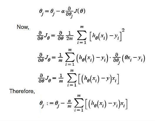
    For a prediction y_hat = w·x + b and loss MSE = (1/n) Σ (y_hat_i - y_i)²:

        dL/dw = (2/n) Σ (y_hat_i - y_i) * x_i
        dL/db = (2/n) Σ (y_hat_i - y_i)

        Update every step with learning rate α:
        w := w - α * dL/dw
        b := b - α * dL/db

        # numpy version
        for _ in range(epochs):
            err = X @ w + b - y
            w -= lr * (2 / n) * X.T @ err
            b -= lr * (2 / n) * err.sum()

    Scale the features first. Otherwise the loss surface is elongated and gradient descent zig-zags or diverges.
    A Support Vector Machine finds the hyperplane that separates the classes with the maximum margin, meaning the largest
    distance to the nearest training points. Those nearest points are the support vectors, and only they determine the
    boundary. The soft-margin SVM allows some violations, traded off by C (large C gives a narrower margin and fewer
    violations, so more variance). Equivalently, it minimises hinge loss plus an L2 penalty. With the kernel trick
    (RBF, polynomial) it learns non-linear boundaries without computing the high-dimensional features explicitly.
    SVR is the regression variant.

    SVM vs OvR is not a like-for-like comparison. An SVM is a binary classifier. One-vs-Rest (OvR) and One-vs-One (OvO)
    are strategies for turning any binary classifier into a multi-class one:
        * OvR: train K classifiers ("class k vs everything else") and predict the class with the highest score.
          This needs K models, and each one sees imbalanced data.
        * OvO: train K(K-1)/2 classifiers, one per pair of classes, and take a majority vote.
          There are more models, but each is trained on a small subset. scikit-learn's SVC uses OvO internally.
    Models that are natively multi-class need neither strategy: decision trees, random forests, kNN, naive Bayes,
    multinomial logistic regression, and neural networks with a softmax output.

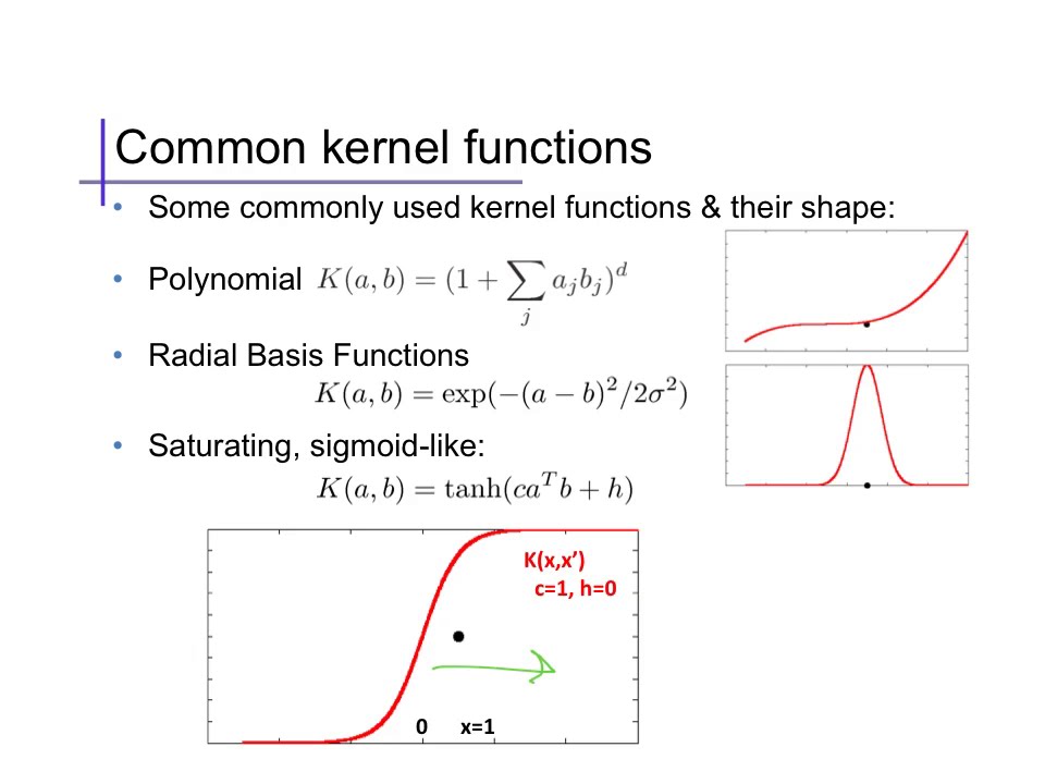
    A kernel K(x, z) computes the dot product of x and z in some feature space without building that space explicitly.

        1) Linear:      K = x·z                      high-dimensional sparse data (text); fastest; use as a baseline
        2) Polynomial:  K = (γ x·z + r)^d            captures feature interactions up to degree d
        3) RBF/Gaussian: K = exp(-γ ||x - z||²)       default choice for non-linear data; γ controls how local the fit is
        4) Sigmoid:     K = tanh(γ x·z + r)          resembles a neural-network unit; rarely used and not always a valid kernel
        5) Laplacian:   K = exp(-γ ||x - z||₁)        similar to RBF, but less smooth

    Tune C and γ together (grid search on a log scale). A large γ with a large C overfits.
    Kernel SVMs scale roughly O(n²) to O(n³) in the number of samples. Above about 100k rows, use a linear SVM or gradient boosting.
    1) MSE  - mean of squared errors. Differentiable and punishes large errors heavily. Units are squared.
    2) RMSE - sqrt(MSE). Same units as the target, so it is easier to explain.
    3) MAE  - mean of absolute errors. Robust to outliers. It is minimised by predicting the median.
    4) R²   - 1 - SS_res / SS_tot: the fraction of variance explained compared with always predicting the mean. It can be negative.
    5) MAPE - mean(|error| / |y|). Scale-free, but undefined at y = 0 and biased towards under-prediction.
    6) sMAPE / WAPE - variants of MAPE that behave better near zero (common in forecasting).
    7) Huber loss - quadratic for small errors and linear for large ones, which makes it a compromise between MSE and MAE.
    8) Quantile (pinball) loss - used when you need prediction intervals or asymmetric costs.

    MAE : Use MAE when you are doing regression and don’t want outliers to play a big role. It can also be useful if you know that your distribution is multimodal, and it’s desirable to have predictions at one of the modes, rather than at the mean of them.
    MSE : use MSE the other way around, when you want to punish the outliers.
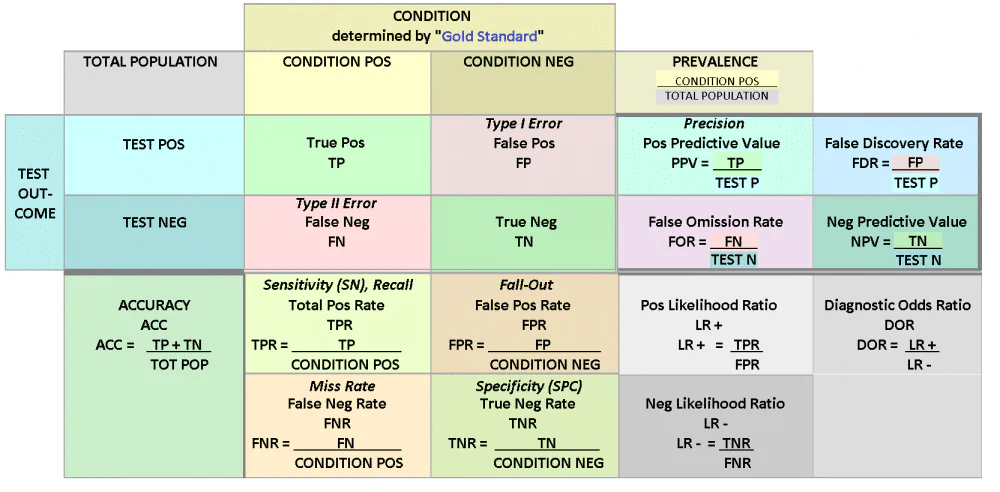
    Start from the confusion matrix (TP, FP, TN, FN), then choose metrics that match the business cost of each error:
        * Accuracy: only meaningful when the classes are balanced.
        * Precision, Recall, F1 (or F-beta to weight recall more heavily).
        * ROC-AUC: threshold-independent ranking quality. PR-AUC is better when positives are rare.
        * Log loss / Brier score and a calibration curve, when the probabilities themselves are used.
        * Per-class and per-segment metrics, since an overall score can hide a failing subgroup.
    Use stratified k-fold cross-validation (or a time-based split for temporal data), and compare against a trivial baseline.
    Choose the decision threshold on validation data, based on the cost of an FP compared with an FN.
    Classification is defined as categorizing classes or entities based on the specified categories either that category exists or not in the respectable data. The concept is quite common for Image based classification or Data Based Classification. The answer in form of Yes or No;
    alongside answers in form of types of objects/classes.
    Multi-class: each example belongs to exactly one of K > 2 classes (for example cat OR dog OR bird).
        Output layer: softmax over K classes. Loss: categorical cross-entropy. Predict the argmax.
    Multi-label: each example can have any subset of the labels (a photo tagged "beach" AND "sunset" AND "people").
        Output layer: K independent sigmoids. Loss: binary cross-entropy per label. Threshold each label separately.
    Metrics also differ. Multi-class uses accuracy and macro/micro F1. Multi-label uses per-label F1, Hamming loss,
    subset accuracy, and mAP.

    A confusion matrix, also known as an error matrix, is a specific table layout that allows visualization of
     the performance of an algorithm, typically a supervised learning one (in unsupervised learning it is
      usually called a matching matrix). Each row of the matrix represents the instances in a predicted class
       while each column represents the instances in an actual class (or vice versa).
    The name stems from the fact that it makes it easy to see if the system is confusing two classes
    (i.e. commonly mislabeling one as another).
    Bias comes from the simplifying assumptions a model makes about the shape of the target function.
        High-bias examples: linear regression, logistic regression, LDA, naive Bayes, shallow trees and decision stumps,
        and kNN with a very large k. They assume linear or otherwise simple boundaries, or independent features.
    They underfit when the true relationship is non-linear or has interactions. Fix that with feature engineering
    (polynomial terms, interactions), kernels, or more flexible models.
    Variance is how much the learned function changes when the training data changes.

        1) High variance (flexible, low bias): fully grown decision trees, kNN with small k, SVMs with RBF and a large C or γ,
           high-degree polynomials, and deep neural networks without regularisation.
        2) Low variance (rigid, higher bias): linear and logistic regression, LDA, naive Bayes, kNN with large k.

    Most algorithms have a knob that moves them along this tradeoff: tree depth, k, C and γ, regularisation strength.
    Ensembles cut variance (bagging) or bias (boosting).
    Linear machine learning algorithms often have a high bias but a low variance.
    Nonlinear machine learning algorithms often have a low bias but a high variance.
    Possible root causes of prediction bias are:

    1) Incomplete feature set
    2) Noisy data set
    3) Buggy pipeline
    4) Biased training sample
    5) Overly strong regularization
    Gradient Descent is an iterative method to solve the optimization problem. There is no concept of "epoch" or "batch" in classical gradient decent. The key of gradient decent are
    * Update the weights by the gradient direction.
    * The gradient is calculated precisely from all the data points.
    Stochastic Gradient Descent can be explained as:
    * Quick and dirty way to "approximate gradient" from one single data point.
    * If we relax on this "one single data point" to "a subset of data", then the concepts of batch and epoch come.

    A decision tree recursively splits the data on the feature and threshold that most reduce impurity (Gini or entropy for
    classification, variance for regression). Each leaf predicts the majority class or the mean value. Trees are
    interpretable, need no feature scaling, and handle non-linearity. A single deep tree has high variance.

    A random forest is a bagged ensemble of decision trees:
        * each tree is trained on a bootstrap sample of the rows, and
        * each split considers only a random subset of features (about sqrt(p) for classification).
    This decorrelates the trees. Averaging their predictions (a majority vote for classification) cuts variance while
    keeping bias low. Rows left out of each bootstrap sample (out-of-bag) give a free validation estimate.
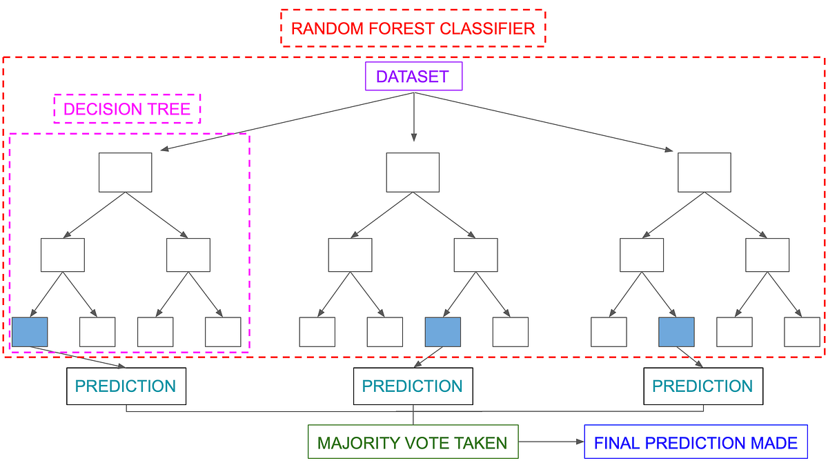
    Splitting is how a decision tree grows. At each node it tries candidate (feature, threshold) pairs and picks the one
    that most reduces impurity in the child nodes: Gini or entropy for classification, variance (MSE) for regression.
    It then recurses on each child until a stopping rule is reached: max depth, min samples per leaf, or no gain.
    Numeric features are split at thresholds between sorted values. Histogram-based methods (LightGBM) bin the values
    first for speed.
    (In the data sense, "splitting" also means dividing data into train, validation and test sets.)
    The shortening of branches of Decision Trees is termed as pruning. The process is done in order to reach the decision earlier than
    expected, reducing the size of the tree by turning some branch nodes into leaf nodes, and removing the leaf nodes under the original branch.
    Tree selection is mainly done from the following
    1) Entropy
            A decision tree is built top-down from a root node and involves partitioning the data into subsets that contain instances with similar
            values (homogeneous). ID 3 algorithm uses entropy to calculate the homogeneity of a sample. If the sample is completely homogeneous the
            entropy is zero and if the sample is an equally divided it has entropy of one.
            Entropy(x) -> -p log(p) - qlog(q)  with log of base 2
    2) Information Gain
            The information gain is based on the decrease in entropy after a dataset is split on an attribute. Constructing a decision tree is all about finding attribute that returns the highest information gain (i.e., the most homogeneous branches).

            2.1) Calculate entropy of the target.
            2.2) The dataset is then split on the different attributes. The entropy for each branch is calculated. Then it is added proportionally, to get total entropy for the split. The resulting entropy is subtracted from the entropy before the split. The result is the Information Gain, or decrease in entropy.
            2.3) Choose attribute with the largest information gain as the decision node, divide the dataset by its branches and repeat the same process on every branch.
from collections import Counter
from math import log2

def entropy(labels):
    n = len(labels)
    return -sum((c / n) * log2(c / n) for c in Counter(labels).values())

def information_gain(parent, children):
    n = len(parent)
    weighted = sum(len(ch) / n * entropy(ch) for ch in children)
    return entropy(parent) - weighted

print(entropy(["a", "a", "b", "b"]))                            # 1.0
print(information_gain(["a", "a", "b", "b"], [["a", "a"], ["b", "b"]])) # 1.0 (perfect split) -* Decision Tree *- A Simple Tree compromising of the process defined in selection of Trees.
-* RandomForest *- Combination of Multiple N number of Decision Trees and using the aggregation to determine the final outcome.
The classifier outcome is based on Voting of each tree within random forest while in case of regression it is based on the
averaging of the tree outcome.
    The Gini Index is calculated by subtracting the sum of the squared probabilities of each class from one. It favors larger partitions.
    Imagine, you want to draw a decision tree and wants to decide which feature/column you should use for your first split?, this is probably defined
    by your gini index.
    Gini Index:
    for each branch in split:
        Calculate percent branch represents .Used for weighting
        for each class in branch:
            Calculate probability of class in the given branch.
            Square the class probability.
        Sum the squared class probabilities.
        Subtract the sum from 1. #This is the Ginin Index for branch
    Weight each branch based on the baseline probability.
    Sum the weighted gini index for each split.
    Favors larger partitions.
    Uses squared proportion of classes.
    Perfectly classified, Gini Index would be zero.
    Evenly distributed would be 1 - (1/# Classes).
    You want a variable split that has a low Gini Index.
    The algorithm works as 1 - ( P(class1)^2 + P(class2)^2 + … + P(classN)^2)
    Probability treats the parameters as fixed and asks how likely the data is:
    "if the coin is fair (p = 0.5), what is the chance of 7 heads in 10 tosses?"

    Likelihood treats the observed data as fixed and asks how well each parameter value explains it. It is the same formula,
    read as a function of the parameter: L(p | data) = P(data | p). It is not a probability distribution over p,
    because it does not have to sum to 1.

    Binomial example with 7 heads in 10 tosses:
        L(p) = C(10, 7) * p^7 * (1 - p)^3
        L(0.5) = 120 * 0.5^10 ≈ 0.117
        L(0.7) = 120 * 0.7^7 * 0.3^3 ≈ 0.267   <- p = 0.7 explains the data better
    In general, for k successes in n trials: L(p) = C(n, k) * p^k * (1 - p)^(n - k).
    Maximum likelihood estimation picks the p that maximises L, which here is p_hat = k/n = 0.7.
    Entropy measures the impurity or uncertainty of a label distribution:
        H(S) = -Σ p_k * log2(p_k)
    It is 0 for a pure node and 1 bit for a 50/50 binary split.

    Information gain is the reduction in entropy produced by a split:
        IG(S, A) = H(S) - Σ_v (|S_v| / |S|) * H(S_v)
    A decision tree picks the split with the highest information gain.

    The difference: entropy describes one set, while information gain compares a parent set with its children after a split.
    Caveat: information gain favours features with many distinct values (an ID column splits perfectly).
    C4.5 corrects for this with the gain ratio.
    Kullback-Leibler divergence measures how much a distribution Q differs from a reference distribution P:
        KL(P || Q) = Σ P(x) * log(P(x) / Q(x))
    It is always >= 0, and equals 0 only when P = Q. It is not symmetric: KL(P||Q) ≠ KL(Q||P).
    It is not a true distance.

    Relationship to cross-entropy: H(P, Q) = H(P) + KL(P || Q). With P fixed (the labels), minimising cross-entropy is
    the same as minimising KL.

    Use cases:
        * VAEs: a KL term pulls the latent posterior towards the prior.
        * Knowledge distillation: a student matches the teacher's soft output distribution.
        * RLHF / PPO / DPO: a KL penalty keeps the fine-tuned policy close to the reference model.
        * Drift monitoring: compare feature distributions between training and production (often via the symmetric JS divergence).
        * t-SNE minimises KL between neighbour distributions in high and low dimensions.

    Entropy: Randomness of information being processed.

    Cross Entropy: A measure from the field of information theory, building upon entropy and generally calculating the difference between two
    probability distributions. It is closely related to but is different from KL divergence that calculates the relative entropy between two
    probability distributions, whereas cross-entropy can be thought to calculate the total entropy between the distributions.

    Cross-entropy can be calculated using the probabilities of the events from P and Q, as follows:
            H(P, Q) = -sum x in X P(x) * log(Q(x))
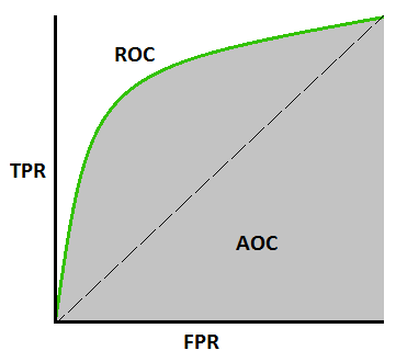
    ROC is a probability curve and AUC represents degree or measure of separability. AUC - ROC curve is a performance measurement for classification problem at various thresholds settings.

    It tells how much model is capable of distinguishing between classes. Mainly used in classification problems for measure at different thresholds.
    Higher the AUC, better the model is at predicting 0s as 0s and 1s as 1s. By analogy, Higher the AUC, better the model is at distinguishing between patients with disease and no disease.
    False positive (Type I error): the actual class is negative, but the model predicts positive.
        Example: a legitimate email flagged as spam, or a healthy patient diagnosed as sick.

    False negative (Type II error): the actual class is positive, but the model predicts negative.
        Example: a fraudulent transaction approved, or a sick patient told they are healthy.

    In hypothesis testing, α = P(Type I) (the significance level) and β = P(Type II). Power = 1 - β.
    Lowering the decision threshold trades FNs for FPs, and raising it does the opposite.
    Take a simple Classification example of "Classifying email messages as spam or not spam"

    Precision measures the percentage of emails flagged as spam that were correctly classified, that is, the percentage of dots to the right of the threshold line, it is also defined as % of event being Called at positive rates e.g
            Precision = True Positive / (True Positive + False positive)

    Recall measures the percentage of actual spam emails that were correctly classified
            Recall = True Postives / (True Positive + False Negative)

    There is always a tradeoff between precision and Recall same is the case of Bias and Variance.
    This totally depends on Business Usecase or SME usecase. In case of Fraud Detection Business domains such as banks, online ecommerce websites
    recommends of better recall score than precision. While in other cases such as word suggestions or Multi label Categorization it can be precision.
    In general, totally dependent on your use case.
    F1 = 2 * Precision * Recall / (Precision + Recall), which is the harmonic mean of precision and recall.
    It ranges from 0 to 1. For binary sets it equals the Dice coefficient.

    Intuition: the harmonic mean is dominated by the smaller value. A model with precision 1.0 and recall 0.01 gets
    F1 ≈ 0.02, not 0.5. You only score well if both are reasonable. F1 also ignores true negatives, which suits
    imbalanced problems.

    Limitation: F1 weights precision and recall equally. When the costs differ, use F-beta
    (beta > 1 favours recall, beta < 1 favours precision), or better, pick a threshold from an explicit cost model.
    For multi-class problems, state whether you report macro F1 (every class equal), micro F1, or weighted F1.
    Both are linear classifiers of the form sign(w·x + b). The difference is what they optimise.

        * Perceptron: finds any separating hyperplane. Its update rule only fires on misclassified points.
          The solution depends on the order of the data and never converges if the data is not separable.
        * SVM: finds the maximum-margin hyperplane. It minimises hinge loss plus an L2 penalty,
          which gives a unique solution that generalises better.

    Put another way, SVM ≈ hinge loss + L2 regularisation + a margin, while the perceptron uses a "zero-margin" hinge
    loss with no regularisation. Both can be kernelised. Both can be trained online (a linear SVM with SGD or Pegasos),
    although classic kernel SVM solvers such as SMO are batch methods.
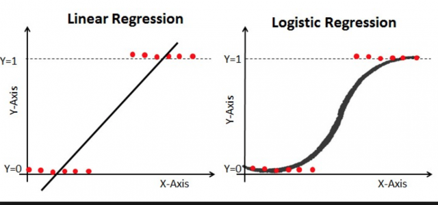
        Linear regression                          | Logistic regression
        ------------------------------------------ | ------------------------------------------
        Predicts a continuous value in (-inf, inf) | Predicts a probability in (0, 1), used for classification
        y = w·x + b                                | P(y=1|x) = sigmoid(w·x + b)
        Loss: mean squared error                   | Loss: log loss (binary cross-entropy)
        Closed-form solution exists                | No closed form; solved iteratively (gradient descent, L-BFGS)
        Coefficient = change in y per unit of x    | Coefficient = change in log-odds per unit of x

    Both are linear models. Logistic regression's decision boundary w·x + b = 0 is a hyperplane.
    An outlier is an observation that lies far from the rest of the data. It can be a data error (sensor glitch, typo)
    or a genuine rare event (fraud, a viral post). Investigate first. Only drop points you can show are errors,
    because in anomaly or fraud problems the outliers are the signal.

    Detection:
        1) IQR rule: flag values outside [Q1 - 1.5*IQR, Q3 + 1.5*IQR]. This is robust and works for skewed data.
        2) Z-score: flag |z| > 3. This assumes roughly normal data, and the outliers themselves inflate the std.
           The modified z-score (based on the median and MAD) is more robust.
        3) Multivariate: Isolation Forest, LOF, Mahalanobis distance.

    Handling (often better than deleting):
        * cap or winsorise at percentiles, or log-transform skewed features
        * use robust models and losses (tree-based models, MAE or Huber loss, RobustScaler)

    Regularization techniques are used to reduce the error by fitting a function appropriately on the given training set and avoid overfitting.
    They add a penalty term (Lambda * weight magnitude) to the loss function to discourage overly complex models.
    1) L1 Regularization (Lasso Regression)
        (Least Absolute Shrinkage and Selection Operator) adds “absolute value of magnitude” of coefficient as penalty term to the loss function.

    2) L2 Regularization (Ridge Regression)
        Adds “squared magnitude” of coefficient as penalty term to the loss function. Here the highlighted part represents L2 regularization element.

    The key difference between these techniques is that Lasso shrinks the less important feature’s coefficient to zero thus, removing some feature
    altogether. So, this works well for feature selection in case we have a huge number of features.
    Data Sampling statistical analysis technique used to select, manipulate and analyze a representative subset of data points to identify patterns and trends in the larger data set being examined.
    There are different techniques of sampling your data
    1) Simple Random Sampling (records are picked at random)
    2) Stratified Sampling (subsets based on common factor with equal ratio distribution)
    3) Cluster Sampling (largest set is breaken down in form of clusters based on defined factors and SRS is applied)
    4) MultiStage Sampling (cluster on Cluster sampling)
    5) Symentaic Sampling (Sample created by setting interval)
    Both rebalance class frequencies in the training set only. Never resample the validation or test set.

    Undersampling removes examples from the majority class. For example, keep 100k of 1M negatives next to 100k positives.
    It is fast, but it throws away information. Variants such as Tomek links and NearMiss remove redundant or borderline points.

    Oversampling adds examples to the minority class, either by duplicating them (random oversampling) or by
    synthesising new ones (SMOTE, ADASYN). It keeps all the data, but duplication can cause overfitting.

    Resampling changes the base rate, so predicted probabilities become miscalibrated. Recalibrate them, or correct
    for the sampling rate, before using the scores as probabilities.
    Imbalancment is when you don't have balance in between classes.
    Imabalnced class is when the normal distribution/support count of multiple classes or classes being considered are not the same or almost same.
    E.G:
        Class A has 1 Million Record
        Class B has 1000 Record
    This is imbalanced data set and Class B is UnderBalanced Class.
        1) Use the right metrics first: PR-AUC, recall at a fixed precision, F1. Never plain accuracy.
        2) Class weights in the loss (class_weight="balanced", scale_pos_weight in XGBoost). This is often the simplest fix.
        3) Resampling of the training data only: undersampling, oversampling, SMOTE.
        4) Tune the decision threshold on validation data instead of using 0.5.
        5) Focal loss (deep learning) to focus training on hard examples.
        6) Collect more minority examples, or use data augmentation.
        7) For extreme imbalance, frame the problem as anomaly detection.
    Use stratified splits so every fold contains positives.
    A moving average smooths a time series by averaging the last n points. A weighted moving average gives each point in
    the window a different weight, usually larger for recent points, so it reacts faster to changes:

        WMA_t = Σ_{i=0..n-1} w_i * x_{t-i} / Σ w_i        e.g. weights n, n-1, ..., 1

    The exponential moving average (EMA) is the most common version. Its weights decay geometrically:
        EMA_t = α * x_t + (1 - α) * EMA_{t-1}
    Use cases: trend smoothing, simple forecasting baselines, technical indicators, and the momentum and Adam optimisers
    (which keep an EMA of gradients).
    ARIMA(p, d, q) = AutoRegressive Integrated Moving Average, a classical univariate forecasting model.
        * AR(p): regress on the last p values of the series.
        * I(d):  difference the series d times to make it stationary (remove the trend).
        * MA(q): regress on the last q forecast errors.
    Choose d with stationarity tests (ADF, KPSS). Choose p and q from the PACF and ACF plots, or by AIC (auto_arima).
    SARIMA adds seasonal terms, and ARIMAX / SARIMAX add external regressors.
    ARIMA is a strong baseline for a single short series. For many related series, gradient boosting on lag features or
    global deep-learning models usually does better.
    Bagging (bootstrap aggregating): train many models independently, in parallel, on bootstrap samples of the data,
    then average or vote. It reduces variance, so it suits high-variance base learners such as deep trees. Example: random forest.

    Boosting: train models sequentially, each one correcting the errors of the ensemble so far. AdaBoost reweights
    misclassified samples. Gradient boosting fits each new tree to the negative gradient of the loss (the residuals).
    It mainly reduces bias and uses shallow trees. Examples: XGBoost, LightGBM, CatBoost.

    XGBoost vs Random Forest:
        * Sequential vs parallel tree building. Shallow trees vs deep trees.
        * XGBoost has a learning rate, L1/L2 regularisation on leaf weights, native missing-value handling,
          and second-order (Hessian) optimisation.
        * XGBoost usually achieves higher accuracy on tabular data, but needs more tuning and can overfit.
          Random forest is robust with default settings and hard to overfit by adding more trees.
    The interquartile range is the spread of the middle 50% of the data: IQR = Q3 - Q1, where
        Q1 = 25th percentile, Q2 = 50th percentile (the median), Q3 = 75th percentile.
    The quartiles are cut points, not ranges.

    Outlier rule (Tukey's fences): flag x < Q1 - 1.5*IQR or x > Q3 + 1.5*IQR. Use 3*IQR for "extreme" outliers.
    The whiskers of a box plot are drawn this way. Because the rule uses percentiles, it is robust to the outliers
    themselves, unlike the z-score.

        q1, q3 = np.percentile(x, [25, 75]); iqr = q3 - q1
        mask = (x >= q1 - 1.5 * iqr) & (x <= q3 + 1.5 * iqr)
    SMOTE (Synthetic Minority Over-sampling TEchnique) creates new minority-class examples instead of duplicating existing ones:
        1) pick a minority sample x
        2) find its k nearest minority-class neighbours (k = 5 by default)
        3) create a synthetic point x_new = x + λ * (neighbour - x), with λ ~ Uniform(0, 1)
    So the new points lie on line segments between minority samples.

    Caveats:
        * Apply it only to the training folds, inside the cross-validation pipeline (imblearn.pipeline). Otherwise it leaks.
        * It can create noisy points in overlapping regions, and it works poorly in very high dimensions.
        * It needs numeric features. For categorical features use SMOTENC.
        * Variants: Borderline-SMOTE, ADASYN, SMOTE-Tomek.
    With strong learners such as gradient boosting, class weights plus threshold tuning often match SMOTE.
    Underfitting (high bias: training error is high):
        1) Use a more complex model, or add capacity (deeper trees, more layers)
        2) Add better features and interactions
        3) Reduce regularisation
        4) Train longer, or fix the learning rate (too high diverges, too low stalls)

    Overfitting (high variance: train error is low but validation error is high):
        1) Get more training data, or use data augmentation
        2) Regularisation: L1/L2 penalties, dropout, weight decay
        3) Early stopping on a validation metric
        4) Simplify the model or remove noisy features
        5) Bagging and ensembles
        6) Use cross-validation to detect it and to tune the hyperparameters above
    1) More data, or data augmentation
    2) L1 / L2 regularisation and weight decay
    3) Dropout (neural networks)
    4) Early stopping
    5) Simpler models: shallower trees, fewer features, pruning
    6) Ensembling (bagging, random forests)
    7) Cross-validation for honest model selection
    8) Batch normalisation and label smoothing (mild regularisers in deep learning)
    A "neuron" in an artificial neural network is a mathematical approximation of a biological neuron.
    It takes a vector of inputs, performs a transformation on them, and outputs a single scalar value.
     It can be thought of as a filter. Typically we use nonlinear filters in neural networks.

    1) Input Layer: Initial input for your neural network
    2) Hiddent layers: a hidden layer is located between the input and output of the algorithm,
    in which the function applies weights to the inputs and directs them through an activation function as the output.
    In short, the hidden layers perform nonlinear transformations of the inputs entered into the network.
    Hidden layers vary depending on the function of the neural network, and similarly, the layers may vary depending
    on their associated weights.
    The output layer turns the last hidden representation into the prediction. Its activation and loss must match the task:
        Regression                 -> linear (no activation), MSE / MAE / Huber loss
        Binary classification      -> 1 unit with sigmoid, binary cross-entropy
        Multi-class classification -> K units with softmax, categorical cross-entropy
        Multi-label classification -> K units with sigmoid each, binary cross-entropy per label
        Positive-only targets      -> softplus or exp (e.g. counts, variances)
    ReLU is a hidden-layer activation. It is rarely the right output activation.
    In PyTorch, output raw logits and use CrossEntropyLoss or BCEWithLogitsLoss, which apply softmax or sigmoid
    internally in a numerically stable way.
    An activation function adds non-linearity after each linear layer. Without it, any stack of linear layers collapses
    into a single linear map, however deep the network is.
    Common choices:
        1) Sigmoid: squashes to (0, 1). Used for binary and multi-label outputs and LSTM gates. It saturates at both
           ends, which causes vanishing gradients in deep hidden layers.
        2) Softmax: turns a vector of logits into a probability distribution that sums to 1. Used for the multi-class
           output layer (mutually exclusive classes).
        3) Tanh: squashes to (-1, 1) and is zero-centred. It also saturates. Used for RNN hidden states.
        4) ReLU: max(0, x). Cheap, and does not saturate for x > 0. The default for hidden layers.
           Units can "die" if they only ever receive negative inputs.
        5) Leaky ReLU / PReLU / ELU: a small slope or smooth curve for x < 0, which avoids dead units.
        6) GELU / SiLU (Swish): smooth ReLU-like functions, standard in transformers and LLMs.
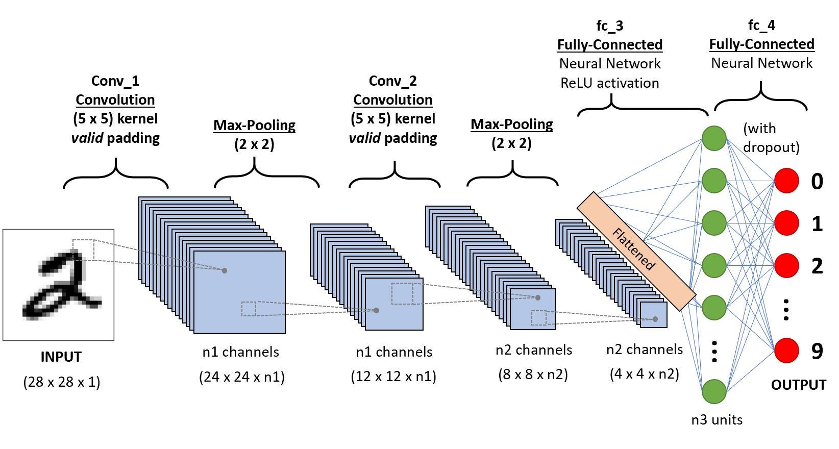
    convolutional-neural-network is a subclass of neural-networks which have at least one convolution layer.
    They are great for capturing local information (e.g. neighbor pixels in an image or surrounding words in a text)
    as well as reducing the complexity of the model (faster training, needs fewer samples, reduces the chance of overfitting).
    . A convolution unit receives its input from multiple units from the previous layer which together create a proximity.
    Therefore, the input units (that form a small neighborhood) share their weights.
    A class of artificial neural networks where connections between nodes form a directed graph along a temporal sequence.
    This allows it to exhibit temporal dynamic behavior. Derived from feedforward neural networks, RNNs can use their
    internal state (memory) to process variable length sequences of inputs. This makes them applicable to tasks such
    as unsegmented, connected handwriting recognition or speech recognition.

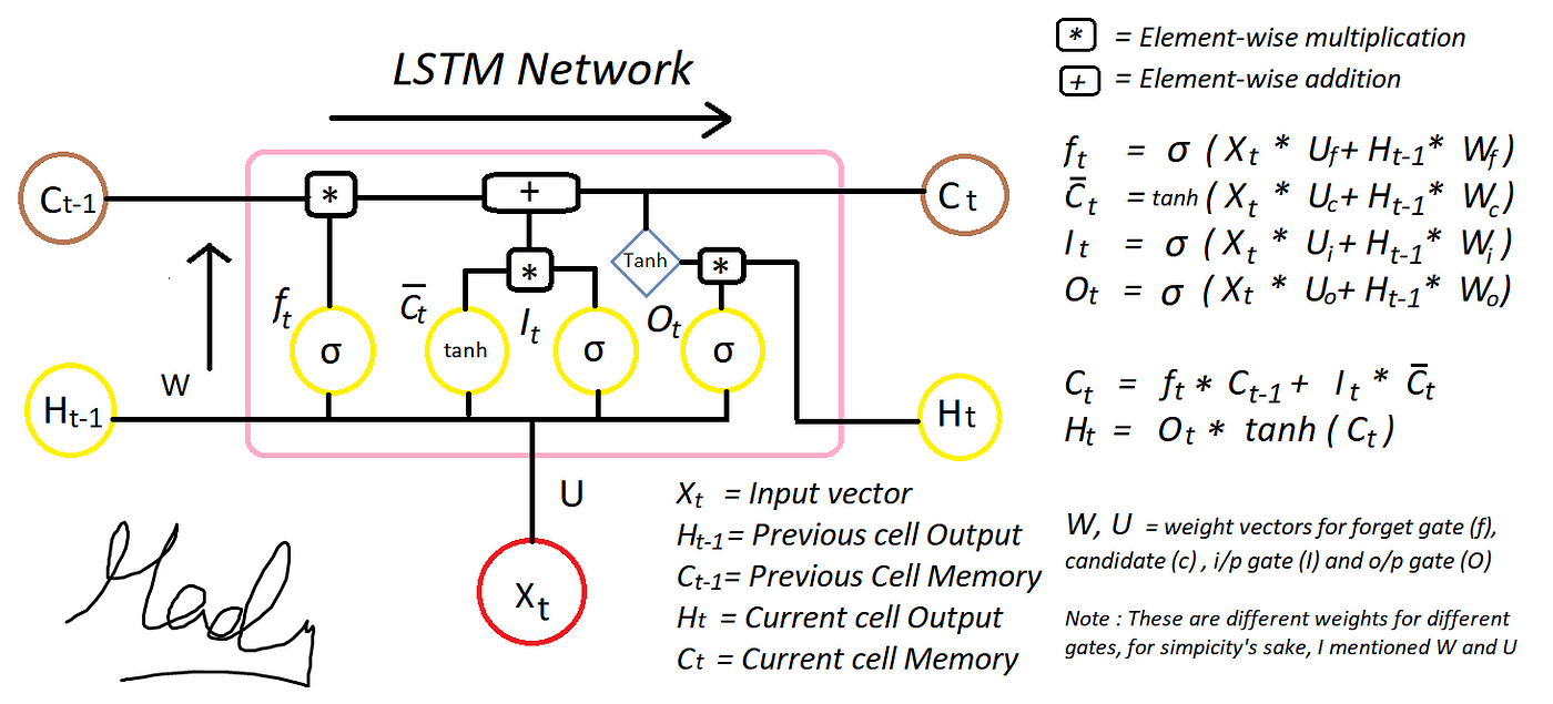
    Long Short-Term Memory (LSTM) is a recurrent neural network cell built to learn long-range dependencies that vanilla
    RNNs forget because of vanishing gradients. It keeps a separate cell state that is updated additively, and three
    sigmoid gates control it: forget (what to erase), input (what to write), and output (what to expose as the hidden
    state). Because the additive path lets gradients flow across many time steps, it can remember information for
    hundreds of steps.
    Use cases: speech recognition, handwriting recognition, time-series forecasting, anomaly detection on sequences,
    and machine translation before transformers. Transformers have largely replaced LSTMs for language, but LSTMs remain
    useful for small, streaming, or on-device sequence models.
    A convolution is the simple application of a filter to an input that results in an activation. Repeated application of the
    same filter to an input results in a map of activations called a feature map, indicating the locations and strength of a
    detected feature in an input, such as an image.
    You can use Filters which are based on Horizental Lines or Verticial Lines or Gray Scale conversion or other conversion filters.

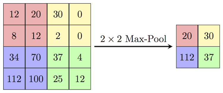
    Pooling layers provide an approach to down sampling feature maps by summarizing the presence of features in patches of the feature map.
    Two common pooling methods are average pooling and max pooling that summarize the average presence of a feature and the most activated
    presence of a feature respectively.

    This is required to downsize your feature scale (e.g You have detected vertical lines, now remove some of the feature to go in grain)

Max pooling uses the maximum value found in a considered region. Maximum pooling, or max pooling, is a pooling operation that calculates the maximum, or largest, value in each patch of each feature map.
    The word "kernel" means two different things in ML.

    1) In CNNs, a kernel (filter) is a small learned weight tensor, for example 3x3xC_in. It slides over the input and
       computes a dot product at each position, producing one feature map per filter. Early layers learn edge and texture
       detectors. Deeper layers learn parts and objects.

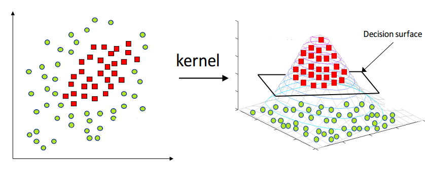
    2) In kernel methods (SVMs, kernel PCA, Gaussian processes), a kernel K(x, z) = φ(x)·φ(z) is a similarity function
       equal to a dot product in some (possibly infinite-dimensional) feature space. The "kernel trick" lets a linear
       algorithm learn non-linear boundaries without ever computing φ(x). Common kernels are linear, polynomial and RBF.
    Segmentation partitions an input into meaningful regions, at the pixel level for images:
        * Semantic segmentation: a class for every pixel.
        * Instance segmentation: a separate mask for each object instance.
        * Panoptic segmentation: both at once.
    The same word also appears elsewhere: customer segmentation (clustering users), and text or audio segmentation
    (splitting a stream into sentences, speakers, or events).
    Pose estimation predicts the positions of an object's keypoints. For humans these are joints such as shoulders,
    elbows and knees, in 2D image coordinates or in 3D. Top-down methods detect each person and then find keypoints
    (HRNet, ViTPose). Bottom-up methods find all keypoints and then group them into people (OpenPose).
    Keypoints are usually predicted as heatmaps.
    Uses: fitness apps, motion capture, AR, sign language, and action recognition.
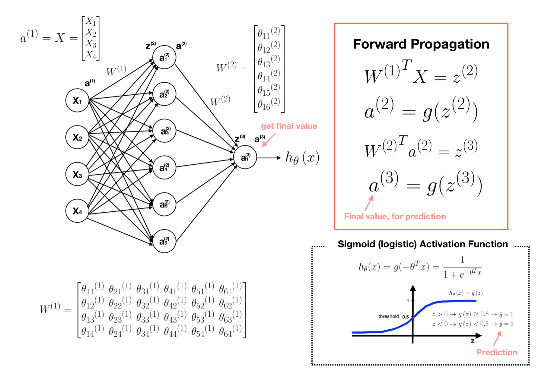
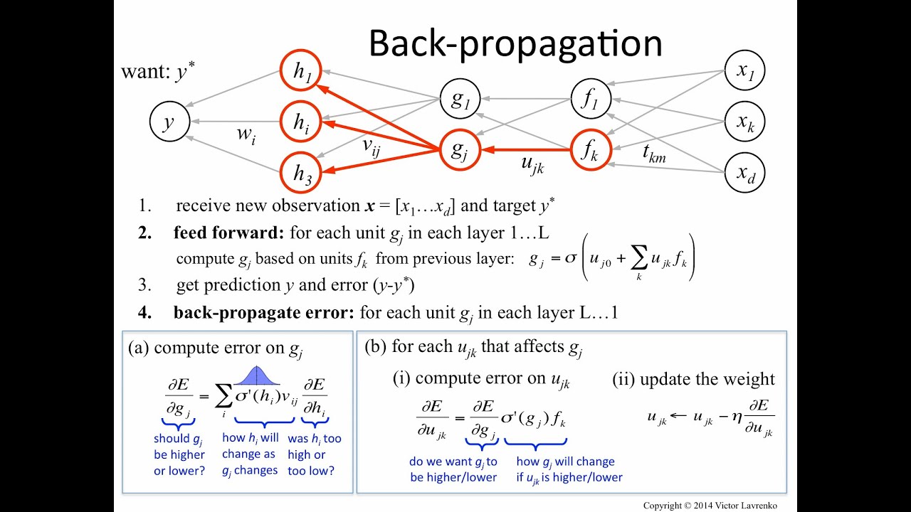
    The input data is fed in the forward direction through the network. Each hidden layer accepts the input data,
    processes it as per the activation function and passes to the successive layer.
    Backpropagation computes the gradient of the loss with respect to every weight by applying the chain rule backwards
    through the network, from the output layer to the input (reverse-mode automatic differentiation). It reuses the
    intermediate activations from the forward pass, so the whole gradient costs about as much as a couple of forward passes.

    Backprop only computes the gradients. The optimiser (SGD, Adam) then uses them to update the weights,
    w := w - lr * dL/dw. This happens on every mini-batch, not once per epoch.
    The term “dropout” refers to dropping out units (both hidden and visible) in a neural network.
    Simply put, dropout refers to ignoring units (i.e. neurons) during the training phase of certain
    set of neurons which is chosen at random. By “ignoring”, I mean these units are not considered during
    a particular forward or backward pass.
    More technically, At each training stage, individual nodes are either dropped out of the net with
    probability 1-p or kept with probability p, so that a reduced network is left; incoming and
    outgoing edges to a dropped-out node are also removed.
    A flatten layer collapses the spatial dimensions of the input into the channel dimension.
    For example, if the input to the layer is an H-by-W-by-C-by-N-by-S array (sequences of images),
    then the flattened output is an (H*W*C)-by-N-by-S array.
    The gradient dL/dw tells each weight which direction increases the loss and by how much. Moving every weight a small
    step in the opposite direction lowers the loss on the current mini-batch. Repeating this over many batches makes the
    network's predictions match the targets better.
    Backprop makes this practical: the chain rule gives all gradients in a single backward pass, instead of perturbing
    each of millions of weights one at a time.
    Better training loss improves generalisation only if overfitting is controlled (validation monitoring, regularisation).
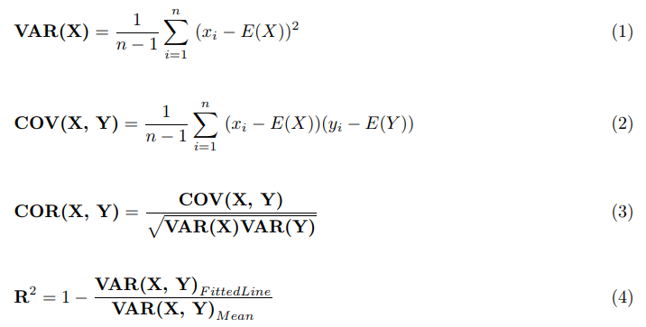
    Covariance measures how two variables vary together:
        cov(X, Y) = E[(X - μx)(Y - μy)]
    Its sign gives the direction of the linear relationship. Its magnitude depends on the units, so it is hard to compare
    across variables.

    Correlation (Pearson) is covariance scaled to [-1, 1]:
        ρ = cov(X, Y) / (σx * σy)
    This makes it unit-free, so it measures both the strength and the direction of the linear relationship.

    Notes:
        * Correlation does not imply causation. A confounder can drive both variables.
        * Pearson only captures linear relationships. Spearman (rank-based) captures monotonic ones and is robust to outliers.
        * A correlation of 0 does not mean the variables are independent (for example, y = x² on symmetric x).
    Analysis of variance (ANOVA) is a collection of statistical models and their associated estimation procedures
    (such as the "variation" among and between groups) used to analyze the differences among group means in a sample.

    Use a one-way ANOVA when you have collected data about one categorical independent variable and
    one quantitative dependent variable. The independent variable should have at least three levels
     (i.e. at least three different groups or categories)
    Dimensionality reduction or dimension reduction is the process of reducing the number of random variables
    under consideration by obtaining a set of principal variables. Approaches can be divided into feature
    selection and feature extraction.
    The reason we use it is because
            1) Immensive dataset
            2) Longer Trainnig time/gathering time
            3) Too much complex assumptions/ Model overfitting
    Types of Dimensionality reductions are
            1) Feature Selection
            2) Feature Projection( transform data from higher dimention to lower space of fewer dimention)
            3) Principle component Analysis
                    Linear Technique for DR, performs linear mapping of data to lower dimention
                    space in such a way variance is maximized.
            4) Non Negative Metrics Factorization
            5) Kernel PCA ( Non linear way of utilization of Kernel Trick)
            6) Graph Based Kernel PCA ( locally linear embedding, Eigen Embeddings)

            7) Linear Discriminant Analysis
                    A method used in statistics, pattern recognition and machine learning to find a
                    linear combination of features that characterizes or separates two or more
                    classes of objects or events.
            8) Generalized Discriminant Analysis
            8) TSNE (is a non-linear dimensionality reduction technique useful for visualization of high-dimensional datasets.)
            9) U-Map
                    Uniform manifold approximation and projection (UMAP) is a nonlinear dimensionality reduction technique.
                    Visually, it is similar to t-SNE, but it assumes that the data is uniformly distributed on a locally
                    connected Riemannian manifold and that the Riemannian metric
                    is locally constant or approximately locally constant.
            10) Autoencoders (can learn from Non Linear dimention reduction function)
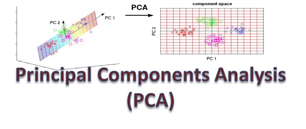
    The main linear technique for dimensionality reduction, principal component analysis, performs
     a linear mapping of the data to a lower-dimensional space in such a way that the variance of
     the data in the low-dimensional representation is maximized. In practice, the covariance (and
     sometimes the correlation) matrix of the data is constructed and the eigenvectors on this
     matrix are computed. The eigenvectors that correspond to the largest eigenvalues (the
     principal components) can now be used to reconstruct a large fraction of the variance of the
     original data. The original space (with dimension of the number of points) has been reduced
     (with data loss, but hopefully retaining the most important variance) to the space spanned by
     a few eigenvectors
    Maximum likelihood estimation is a method that determines values for the parameters of a model.
    The parameter values are found such that they maximise the likelihood that the process described by the model
    produced the data that were actually observed.
    Naive Bayes is a generative classifier based on Bayes' theorem. It makes the "naive" assumption that features are
    conditionally independent given the class:

        P(class | x1..xn) ∝ P(class) * Π P(xi | class)
        predict  argmax_c  [ log P(c) + Σ log P(xi | c) ]

    Training only requires counting (class priors and per-feature likelihoods), so it is very fast and works with little data.
        * GaussianNB for continuous features, MultinomialNB for word counts, BernoulliNB for binary features.
        * Use Laplace (add-one) smoothing so that a word never seen in training does not zero out the whole product.
        * Work in log space to avoid numerical underflow.
    It is a strong baseline for text classification and spam filtering. Its predicted probabilities are usually poorly
    calibrated, because the independence assumption does not hold.


    Bayes' theorem updates a belief after seeing evidence:

        P(A | B) = P(B | A) * P(A) / P(B)
        posterior = likelihood * prior / evidence

    Classic example: a disease has 1% prevalence, and a test has 99% sensitivity and 5% false-positive rate.
        P(disease | +) = 0.99 * 0.01 / (0.99 * 0.01 + 0.05 * 0.99) ≈ 0.167
    A positive result means only about a 17% chance of disease, because the base rate is low.
    This base-rate effect is why precision collapses on rare-event problems such as fraud.
    Probability is a number between 0 and 1, where, roughly speaking, 0 indicates impossibility and 1 indicates certainty.
    The higher the probability of an event, the more likely it is that the event will occur.
    Example:
    A simple example is the tossing of a fair (unbiased)
    coin. Since the coin is fair, the two outcomes ("heads" and "tails") are both equally probable; the probability of "heads" equals the probability
    of "tails"; and since no other outcomes are possible, the probability of either "heads" or "tails" is 1/2 (which could also be written as 0.5 or
    50%).
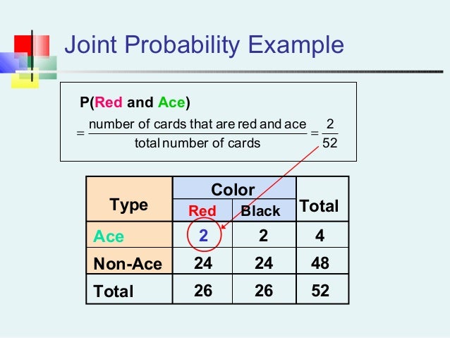
    Joint probability is a statistical measure that calculates the likelihood of two events occurring together and at the same point in time.
            P(A and B) or P (A ^ B) or P(A & B)
            The joint probability is detremeinded as :
            P(A and B) = P(A given B) * P(B)
    Marginal probability is the probability of one variable on its own, regardless of the values of other variables.
    You get it by summing (or integrating) the joint distribution over the other variables:

        P(A) = Σ_b P(A, B = b)

    Example: if the joint table gives P(rain, weekend) and P(rain, weekday), then
    P(rain) = P(rain, weekend) + P(rain, weekday). It is called "marginal" because these totals used to be written in the
    margins of the table.
    Conditional probability is the probability of A given that B has happened:
        P(A | B) = P(A, B) / P(B),  defined when P(B) > 0
    A and B are independent if and only if P(A | B) = P(A).

    A probability distribution assigns probabilities to every possible value of a random variable.
        * Discrete: a probability mass function (Bernoulli, Binomial, Poisson).
        * Continuous: a probability density function (Normal, Exponential, Uniform).
    The cumulative distribution function F(x) = P(X <= x) exists for both.
    The z-score says how many standard deviations a value lies from the mean: z = (x - μ) / σ.
    Uses: standardising features, outlier flagging (|z| > 3), comparing values on different scales, and
    z-tests in hypothesis testing.
    Under a normal distribution about 68% / 95% / 99.7% of values fall within 1 / 2 / 3 standard deviations.
    The z-score is sensitive to outliers, because they inflate σ. The robust version uses the median and MAD.
    k-Nearest Neighbours is a lazy, instance-based method. Training just stores the data. To predict a new point:
        1) compute its distance to every training point
        2) take the k closest points
        3) classification: majority vote (optionally weighted by 1/distance). Regression: average of their targets.

    The neighbour criterion has two parts, and both can be changed:
        * the distance metric: Euclidean (default), Manhattan, Minkowski-p, cosine (for text and embeddings), Hamming
        * k: a small k gives a noisy boundary (high variance), a large k gives a smooth boundary (high bias).
          Tune k with cross-validation, and use an odd k for binary problems to avoid ties.

    Practical notes: scale the features first, because distances are dominated by large-range features.
    Prediction costs O(n·d) per query, so use KD-trees or ball trees, or approximate nearest-neighbour indexes (FAISS, HNSW)
    at scale. kNN degrades in high dimensions because of the curse of dimensionality.
    Recommended is low FN's, the reason is because if you consider Fraudly Transaction being occured and counting it as not being occured
    This has huge impact on the Business model.
        KNN                                         | K-Means
        ------------------------------------------- | ------------------------------------------------
        Supervised (classification / regression)    | Unsupervised (clustering)
        k = number of neighbours used to vote        | k = number of clusters to find
        No training; all work happens at prediction | Iterative training: assign points to the nearest
                                                    |   centroid, then recompute centroids until stable
        Needs labels                                | Needs no labels
        Output: a label or value for each query     | Output: k centroids plus a cluster id per point
    The only thing they share is distance computation.
    Attention lets a model compute each output as a weighted average over its inputs, with the weights computed from
    how relevant each input is to the current query:
        Attention(Q, K, V) = softmax(Q·Kᵀ / sqrt(d_k)) · V
    Examples:
        * Machine translation (Bahdanau attention): while generating each target word, the decoder attends to the most
          relevant source words instead of squeezing the whole sentence into one vector.
        * Self-attention in transformers: every token attends to every other token in the same sequence.
          "it" in "The animal didn't cross the street because it was tired" attends strongly to "animal".
        * Image captioning ("Show, Attend and Tell"): the model attends to image regions as it generates each word.
    Soft attention (differentiable weights over all inputs) is the standard. Hard attention picks one location and needs
    sampling or RL to train.

    Autoencoders: an encoder compresses the input into a low-dimensional code (the bottleneck), and a decoder
    reconstructs the input from that code. Training minimises reconstruction loss, so no labels are needed.
        * Uses: dimensionality reduction, denoising (denoising autoencoders), anomaly detection
          (a high reconstruction error flags unusual inputs), and pretraining.
        * A variational autoencoder (VAE) makes the code a probability distribution, which turns the model into a generative model.

    Transformers: a sequence architecture built from self-attention instead of recurrence. Every token attends to every
    other token, with attention weights softmax(QKᵀ / sqrt(d)). Each layer stacks multi-head attention and a feed-forward
    network, with residual connections and layer normalisation. Positional encodings supply word order.
    Transformers process all tokens in parallel and model long-range dependencies well. They are the basis of BERT
    (encoder-only), GPT and other LLMs (decoder-only), T5 (encoder-decoder), and Vision Transformers.
    See deep_learning/intro_transformers.md for the full guide.
    Image Captioning is the process of generating textual description of an image. It uses both Natural Language Processing and Computer Vision to
    generate the captions

    Summarization is the task of condensing a piece of text to a shorter version, reducing the size of the initial text while preserving the meaning.
    Some examples are :
            1) Essay Summarization
            2) Document Summarization
            etc
    Style transfer is a computer vision technique that applies the artistic style of one image to the content of another.
    It uses convolutional neural networks (typically VGG) to separate and recombine the content and style representations
    of two images. The loss function combines a content loss (preserving structure of the content image) with a style loss
    (matching Gram matrix statistics of the style image). Neural Style Transfer was introduced by Gatys et al. (2015).
    Modern approaches use fast style transfer (pre-trained feed-forward networks) for real-time applications.
    Use cases: photo filters, artistic image generation, creative tools.
    Image Segmentation : In digital image processing and computer vision, image segmentation is the process of partitioning a digital image into
    multiple segments (sets of pixels, also known as image objects). The goal of segmentation is to simplify and/or change the representation of
    an image into something that is more meaningful and easier to analyze.

    Pose Analysis:
            The process of determining the location and the orientation of a Human Entity (pose).

    Semantic segmentation assigns a class label to every pixel (road, car, person, sky). It does not separate objects:
    two touching people are one "person" region.
    Typical models are encoder-decoders with skip connections (U-Net, DeepLab with atrous convolutions, SegFormer).
    Loss: per-pixel cross-entropy, often combined with Dice loss for imbalanced classes. Metric: mean IoU (mIoU).

    Instance segmentation detects each individual object and gives it its own pixel mask: person #1, person #2, and so on.
    It combines object detection with segmentation. Mask R-CNN, for example, adds a mask head to Faster R-CNN.
    Background classes such as sky or road are ignored.
    Panoptic segmentation combines both: every pixel gets a class, and every countable object also gets an instance ID.
    Metric: mask AP (average precision over IoU thresholds).
    Imperative (define-by-run / eager): each operation executes immediately, as in ordinary Python. PyTorch eager mode and
    TensorFlow 2 eager mode work this way. It is easy to debug with print and pdb, and control flow is plain Python.

    Symbolic (define-then-run / graph): you first build a computation graph, then compile and execute it. TensorFlow 1.x
    graphs, Theano, and JAX's jit tracing work this way. The whole graph is known in advance, which enables optimisations
    such as operator fusion, memory planning, and export to other runtimes. It is harder to debug.

    Modern frameworks mix the two: write eager code, then compile it (torch.compile, tf.function, jax.jit).

    Text classification assigns one or more predefined labels to a piece of text.
    Approaches, from simple to complex: TF-IDF with logistic regression or naive Bayes (a strong baseline),
    fine-tuned transformers (BERT, DeBERTa), and zero-shot or few-shot classification with an LLM.
    Use cases:
            1) Spam and phishing detection
            2) Sentiment analysis of reviews and social posts
            3) Support-ticket routing and intent detection in chatbots
            4) Topic and news categorisation
            5) Toxicity and content moderation
            6) Language identification

    First ask why the data is missing: completely at random (MCAR), at random given other features (MAR), or not at random (MNAR).
        1) Drop rows or columns: only when missingness is rare and MCAR.
        2) Simple imputation: mean or median (numeric), mode or an "unknown" category (categorical).
        3) Add a missing-indicator feature. The fact that a value is missing is often predictive.
        4) Model-based imputation: KNNImputer, IterativeImputer / MICE, MissForest.
        5) Time series: forward fill, backward fill, or interpolation.
        6) Models that handle missing values natively: XGBoost, LightGBM, CatBoost, and HistGradientBoosting learn a default split direction.
    Always fit the imputer on training data only, inside the pipeline, to avoid leakage.
REFERENCED FROM : https://github.com/andrewekhalel/MLQuestions
1) What's the trade-off between bias and variance? [src]
If our model is too simple and has very few parameters then it may have high bias and low variance. On the other hand if our model has large number of parameters then it’s going to have high variance and low bias. So we need to find the right/good balance without overfitting and underfitting the data. [src]
2) What is gradient descent? [src]
Gradient descent is an optimization algorithm used to find the values of parameters (coefficients) of a function (f) that minimizes a cost function (cost).
Gradient descent is best used when the parameters cannot be calculated analytically (e.g. using linear algebra) and must be searched for by an optimization algorithm.
3) Explain over- and under-fitting and how to combat them? [src]
ML/DL models essentially learn a relationship between its given inputs(called training features) and objective outputs(called labels). Regardless of the quality of the learned relation(function), its performance on a test set(a collection of data different from the training input) is subject to investigation.
Most ML/DL models have trainable parameters which will be learned to build that input-output relationship. Based on the number of parameters each model has, they can be sorted into more flexible(more parameters) to less flexible(less parameters).
The problem of Underfitting arises when the flexibility of a model(its number of parameters) is not adequate to capture the underlying pattern in a training dataset. Overfitting, on the other hand, arises when the model is too flexible to the underlying pattern. In the later case it is said that the model has “memorized” the training data.
An example of underfitting is estimating a second order polynomial(quadratic function) with a first order polynomial(a simple line). Similarly, estimating a line with a 10th order polynomial would be an example of overfitting.
4) How do you combat the curse of dimensionality? [src]
- Feature Selection(manual or via statistical methods)
- Principal Component Analysis (PCA)
- Multidimensional Scaling
- Locally linear embedding
[src]
5) What is regularization, why do we use it, and give some examples of common methods? [src]
A technique that discourages learning a more complex or flexible model, so as to avoid the risk of overfitting. Examples
- Ridge (L2 norm)
- Lasso (L1 norm)
The obvious disadvantage of ridge regression, is model interpretability. It will shrink the coefficients for least important predictors, very close to zero. But it will never make them exactly zero. In other words, the final model will include all predictors. However, in the case of the lasso, the L1 penalty has the effect of forcing some of the coefficient estimates to be exactly equal to zero when the tuning parameter λ is sufficiently large. Therefore, the lasso method also performs variable selection and is said to yield sparse models. [src]
6) Explain Principal Component Analysis (PCA)? [src]
Principal Component Analysis (PCA) is a dimensionality reduction technique used in machine learning to reduce the number of features in a dataset while retaining as much information as possible. It works by identifying the directions (principal components) in which the data varies the most, and projecting the data onto a lower-dimensional subspace along these directions.
7) Why is ReLU better and more often used than Sigmoid in Neural Networks? [src]
- Computation Efficiency: As ReLU is a simple threshold the forward and backward path will be faster.
- Reduced Likelihood of Vanishing Gradient: Gradient of ReLU is 1 for positive values and 0 for negative values while Sigmoid activation saturates (gradients close to 0) quickly with slightly higher or lower inputs leading to vanishing gradients.
- Sparsity: Sparsity happens when the input of ReLU is negative. This means fewer neurons are firing ( sparse activation ) and the network is lighter.
8) Given stride S and kernel sizes for each layer of a (1-dimensional) CNN, create a function to compute the receptive field of a particular node in the network. This is just finding how many input nodes actually connect through to a neuron in a CNN. [src]
The receptive field is the region of the input that can influence one output unit. For a stack of 1-D conv layers
with kernel sizes k_i and strides s_i, each layer adds (k_i - 1) times the product of the strides of all
earlier layers:
def receptive_field(kernels, strides):
    rf, jump = 1, 1              # jump = distance in input pixels between adjacent units
    for k, s in zip(kernels, strides):
        rf += (k - 1) * jump
        jump *= s
    return rf

print(receptive_field([3, 3, 3], [1, 1, 1]))   # 7  (three 3x3 convs == one 7x7)
print(receptive_field([3, 3, 3], [2, 2, 2]))   # 15
Dilation d multiplies the effective kernel size: k_eff = d * (k - 1) + 1.
9) Implement connected components on an image/matrix. [src]
Label each group of touching foreground pixels with a BFS (or union-find) flood fill:
from collections import deque

def connected_components(grid):          # grid: list of lists of 0/1
    h, w = len(grid), len(grid[0])
    labels = [[0] * w for _ in range(h)]
    current = 0
    for i in range(h):
        for j in range(w):
            if grid[i][j] and not labels[i][j]:
                current += 1
                labels[i][j] = current
                q = deque([(i, j)])
                while q:
                    y, x = q.popleft()
                    for dy, dx in ((1, 0), (-1, 0), (0, 1), (0, -1)):   # 4-connectivity
                        ny, nx = y + dy, x + dx
                        if 0 <= ny < h and 0 <= nx < w and grid[ny][nx] and not labels[ny][nx]:
                            labels[ny][nx] = current
                            q.append((ny, nx))
    return labels, current
This runs in O(H·W). The two-pass union-find algorithm is the classic alternative for streaming or hardware use.
10) Implement a sparse matrix class in C++. [src]
Store only the non-zero entries. A dictionary-of-keys (DOK) layout is simplest to build. CSR (compressed sparse row),
which uses three arrays values, col_idx and row_ptr, is best for fast matrix-vector products.
#include <unordered_map>
#include <vector>

class SparseMatrix {
    size_t rows_, cols_;
    std::unordered_map<size_t, double> data_;          // key = r * cols_ + c
public:
    SparseMatrix(size_t r, size_t c) : rows_(r), cols_(c) {}
    void set(size_t r, size_t c, double v) {
        size_t k = r * cols_ + c;
        if (v == 0.0) data_.erase(k); else data_[k] = v;
    }
    double get(size_t r, size_t c) const {
        auto it = data_.find(r * cols_ + c);
        return it == data_.end() ? 0.0 : it->second;
    }
    std::vector<double> multiply(const std::vector<double>& x) const {   // O(nnz)
        std::vector<double> y(rows_, 0.0);
        for (const auto& [k, v] : data_) y[k / cols_] += v * x[k % cols_];
        return y;
    }
};11) Create a function to compute an integral image, and create another function to get area sums from the integral image.[src]
import numpy as np

def integral_image(img):
    # pad with a zero row and column so the queries below need no bounds checks
    ii = np.zeros((img.shape[0] + 1, img.shape[1] + 1), dtype=np.int64)
    ii[1:, 1:] = img.cumsum(0).cumsum(1)
    return ii

def area_sum(ii, top, left, bottom, right):     # inclusive coordinates
    return (ii[bottom + 1, right + 1] - ii[top, right + 1]
            - ii[bottom + 1, left] + ii[top, left])
Building the integral image is O(H·W), and every rectangle sum afterwards is O(1). The Viola-Jones face detector relies on this for Haar features. [Answer]
12) How would you remove outliers when trying to estimate a flat plane from noisy samples? [src]
Random sample consensus (RANSAC) is an iterative method to estimate parameters of a mathematical model from a set of observed data that contains outliers, when outliers are to be accorded no influence on the values of the estimates. [src]
Content-based image retrieval (CBIR) finds images that look like a query image, using the pixels themselves rather than keywords or tags:
- Represent: turn every image into a vector. Older systems used hand-crafted descriptors (colour histograms, SIFT aggregated with bag-of-visual-words, VLAD or Fisher vectors). Modern systems use embeddings from a CNN or ViT, or joint image-text embeddings (CLIP), which also allow text queries.
- Index: store the vectors in an approximate nearest-neighbour index (FAISS, HNSW, IVF-PQ).
- Query: embed the query image, retrieve the top-k nearest vectors by cosine or L2 distance, and optionally re-rank them (geometric verification with keypoint matching and RANSAC, or a heavier model).
Train or fine-tune the embedding with a metric-learning loss (contrastive, triplet) on your own notion of "similar": the same product, a near-duplicate, or the same landmark. Evaluate with recall@k and mAP.
14) How does image registration work? Sparse vs. dense optical flow and so on. [src]
Image registration aligns two images of the same scene into one coordinate frame:
- Detect and describe keypoints (SIFT, ORB, SuperPoint) in both images.
- Match descriptors (nearest neighbour plus Lowe's ratio test).
- Estimate a transform (affine, homography, or a deformable model) robustly with RANSAC.
- Warp one image onto the other, optionally refining by directly optimising an intensity similarity (mutual information for multi-modal medical images).
Sparse vs dense optical flow: sparse flow (Lucas-Kanade) tracks motion only at selected keypoints. It is fast and suited to tracking. Dense flow (Farnebäck, or learned models such as RAFT) estimates a motion vector for every pixel. It is slower, but needed for segmentation, video interpolation, or stabilisation.
15) Describe how convolution works. What about if your inputs are grayscale vs RGB imagery? What determines the shape of the next layer?[src]
In a convolutional neural network (CNN), the convolution operation is applied to the input image using a small matrix called a kernel or filter. The kernel slides over the image in small steps, called strides, and performs element-wise multiplications with the corresponding elements of the image and then sums up the results. The output of this operation is called a feature map.
When the input is RGB(or more than 3 channels) the sliding window will be a sliding cube. The shape of the next layer is determined by Kernel size, number of kernels, stride, padding, and dialation.
16) Talk me through how you would create a 3D model of an object from imagery and depth sensor measurements taken at all angles around the object. [src]
There are two popular methods for 3D reconstruction:
SfM is better suited for creating models of large scenes while MVS is better suited for creating models of small objects.
17) Implement SQRT(const double & x) without using any special functions, just fundamental arithmetic. [src]
Use Newton's method on f(y) = y² - x, which gives the update y ← (y + x / y) / 2. It converges quadratically
(the number of correct digits roughly doubles each step), so it is much faster than a Taylor series:
def sqrt(x, eps=1e-12):
    if x < 0:
        raise ValueError("negative input")
    if x == 0:
        return 0.0
    y = x if x >= 1 else 1.0
    while abs(y * y - x) > eps * x:
        y = 0.5 * (y + x / y)
    return y
For an integer square root, binary search on [0, x] is the other common answer.
[Answer]
18) Reverse a bitstring. [src]
If you are using python3 :
data = b'\xAD\xDE\xDE\xC0'
my_data = bytearray(data)
my_data.reverse()
19) Implement non maximal suppression as efficiently as you can. [src]
Non-Maximum Suppression (NMS) is a technique used to eliminate multiple detections of the same object in a given image. To solve that first sort bounding boxes based on their scores(N LogN). Starting with the box with the highest score, remove boxes whose overlapping metric(IoU) is greater than a certain threshold.(N^2)
To optimize this solution you can use special data structures to query for overlapping boxes such as R-tree or KD-tree. (N LogN) [src]
20) Reverse a linked list in place. [src]
def reverse(head):
    prev = None
    while head:
        head.next, prev, head = prev, head, head.next
    return prev
O(n) time and O(1) extra space. Keep three pointers (prev, current, next) and flip each next pointer as you walk the list.
[Answer]
21) What is data normalization and why do we need it? [src]
Normalization rescales features onto comparable ranges. The two usual forms are standardization
(x - mean) / std and min-max scaling to [0, 1]. It matters because:
- Gradient-based training converges faster. With features on very different scales the loss surface is a long, narrow valley, and gradient descent zig-zags or needs a tiny learning rate.
- Distance- and margin-based models (kNN, k-means, SVM, PCA) depend on it. Without scaling, the feature with the largest range dominates every distance.
- Regularisation treats weights fairly. An L1/L2 penalty only means something if the features share a scale.
Tree-based models (random forests, gradient boosting) don't need it, because their splits are invariant to monotonic rescaling. Always fit the scaler on the training data only and reuse those statistics at validation, test and serving time. Otherwise you leak information, or your features drift between training and serving.
22) Why do we use convolutions for images rather than just FC layers? [src]
Firstly, convolutions preserve, encode, and actually use the spatial information from the image. If we used only FC layers we would have no relative spatial information. Secondly, Convolutional Neural Networks (CNNs) have a partially built-in translation in-variance, since each convolution kernel acts as it's own filter/feature detector.
23) What makes CNNs translation invariant? [src]
Two properties need to be kept apart:
- Convolution is translation-equivariant. The same kernel (shared weights) is applied at every position, so if the input shifts, the feature map shifts by the same amount. A feature detector learned in one corner works everywhere.
- Translation invariance (the output doesn't change when the input shifts) comes from what is stacked on top: pooling, which gives small local invariance, and especially global average pooling or a classifier head that aggregates over all positions.
In practice CNNs are only approximately invariant. Striding and downsampling break exact shift-equivariance, so a shift of a few pixels can change the prediction. Data augmentation with random crops and shifts and anti-aliased downsampling (blur pooling) improve robustness.
24) Why do we have max-pooling in classification CNNs? [src]
Max-pooling downsamples feature maps by keeping the strongest activation in each window (typically 2x2, stride 2):
- Less computation and memory in later layers, because the feature maps are 4x smaller.
- Larger receptive field. Later layers see more of the image, which they need to recognise whole objects.
- Some local translation invariance. A feature that moves a pixel or two within the window gives the same maximum.
- It keeps "is the feature present?" rather than exactly where it is, which is what classification needs.
Many modern architectures replace most pooling with strided convolutions and end with global average pooling. Vision Transformers use patch embeddings instead. For dense tasks such as segmentation, too much pooling hurts localisation, which is why those models use skip connections or dilated convolutions.
25) Why do segmentation CNNs typically have an encoder-decoder style / structure? [src]
The encoder CNN can basically be thought of as a feature extraction network, while the decoder uses that information to predict the image segments by "decoding" the features and upscaling to the original image size.
26) What is the significance of Residual Networks? [src]
Residual networks (ResNets) made very deep networks trainable. Each block learns a residual F(x) and outputs
y = x + F(x) through an identity skip connection.
- Before ResNets, deeper plain networks got worse training error. That rules out overfitting: it was an
optimisation problem (degradation). With a skip connection, a block can easily learn the identity by driving
Fto zero, so adding depth shouldn't hurt. - Gradients flow directly. The gradient of
x + F(x)includes an identity term, so the signal reaches early layers through the skip path without vanishing through dozens of multiplications. - Multiple paths. A ResNet behaves somewhat like an ensemble of many shallower paths of different lengths.
Residual connections are now everywhere. Every transformer layer uses them around attention and the MLP, which is why 100+ layer LLMs train at all.
27) What is batch normalization and why does it work? [src]
Batch normalization normalises each channel's activations using the mini-batch mean and variance, then applies a learned scale and shift:
x_hat = (x - mean_batch) / sqrt(var_batch + eps)
y     = gamma * x_hat + beta
During training it uses batch statistics and updates running averages. At inference it uses those running averages,
so remember to call model.eval().
Why it helps: the original explanation was reducing "internal covariate shift" (layer inputs changing distribution during training). Later work suggests the main effect is a smoother loss landscape, which allows larger learning rates and makes training less sensitive to initialisation. It also regularises a little, because batch statistics are noisy.
Limitations: it behaves badly with small batches, and it adds a train/inference discrepancy. It is awkward for variable-length sequences. That is why transformers use LayerNorm or RMSNorm (per-example statistics), and small-batch vision work uses GroupNorm.
28) Why would you use many small convolutional kernels such as 3x3 rather than a few large ones? [src]
This is very well explained in the VGGNet paper. There are 2 reasons: First, you can use several smaller kernels rather than few large ones to get the same receptive field and capture more spatial context, but with the smaller kernels you are using less parameters and computations. Secondly, because with smaller kernels you will be using more filters, you'll be able to use more activation functions and thus have a more discriminative mapping function being learned by your CNN.
29) Why do we need a validation set and test set? What is the difference between them? [src]
When training a model, we divide the available data into three separate sets:
- The training dataset is used for fitting the model’s parameters. However, the accuracy that we achieve on the training set is not reliable for predicting if the model will be accurate on new samples.
- The validation dataset is used to measure how well the model does on examples that weren’t part of the training dataset. The metrics computed on the validation data can be used to tune the hyperparameters of the model. However, every time we evaluate the validation data and we make decisions based on those scores, we are leaking information from the validation data into our model. The more evaluations, the more information is leaked. So we can end up overfitting to the validation data, and once again the validation score won’t be reliable for predicting the behaviour of the model in the real world.
- The test dataset is used to measure how well the model does on previously unseen examples. It should only be used once we have tuned the parameters using the validation set.
So if we omit the test set and only use a validation set, the validation score won’t be a good estimate of the generalization of the model.
30) What is stratified cross-validation and when should we use it? [src]
Cross-validation is a technique for dividing data between training and validation sets. On typical cross-validation this split is done randomly. But in stratified cross-validation, the split preserves the ratio of the categories on both the training and validation datasets.
For example, if we have a dataset with 10% of category A and 90% of category B, and we use stratified cross-validation, we will have the same proportions in training and validation. In contrast, if we use simple cross-validation, in the worst case we may find that there are no samples of category A in the validation set.
Stratified cross-validation may be applied in the following scenarios:
- On a dataset with multiple categories. The smaller the dataset and the more imbalanced the categories, the more important it will be to use stratified cross-validation.
- On a dataset with data of different distributions. For example, in a dataset for autonomous driving, we may have images taken during the day and at night. If we do not ensure that both types are present in training and validation, we will have generalization problems.
31) Why do ensembles typically have higher scores than individual models? [src]
An ensemble is the combination of multiple models to create a single prediction. The key idea for making better predictions is that the models should make different errors. That way the errors of one model will be compensated by the right guesses of the other models and thus the score of the ensemble will be higher.
We need diverse models for creating an ensemble. Diversity can be achieved by:
- Using different ML algorithms. For example, you can combine logistic regression, k-nearest neighbors, and decision trees.
- Using different subsets of the data for training. This is called bagging.
- Giving a different weight to each of the samples of the training set. If this is done iteratively, weighting the samples according to the errors of the ensemble, it’s called boosting. Many winning solutions to data science competitions are ensembles. However, in real-life machine learning projects, engineers need to find a balance between execution time and accuracy.
32) What is an imbalanced dataset? Can you list some ways to deal with it? [src]
An imbalanced dataset is one that has different proportions of target categories. For example, a dataset with medical images where we have to detect some illness will typically have many more negative samples than positive samples: say, 98% of images are without the illness and 2% of images are with the illness.
There are different options to deal with imbalanced datasets:
- Oversampling or undersampling. Instead of sampling with a uniform distribution from the training dataset, we can use other distributions so the model sees a more balanced dataset.
- Data augmentation. We can add data in the less frequent categories by modifying existing data in a controlled way. In the example dataset, we could flip the images with illnesses, or add noise to copies of the images in such a way that the illness remains visible.
- Using appropriate metrics. In the example dataset, if we had a model that always made negative predictions, it would achieve a precision of 98%. There are other metrics such as precision, recall, and F-score that describe the accuracy of the model better when using an imbalanced dataset.
33) Can you explain the differences between supervised, unsupervised, and reinforcement learning? [src]
In supervised learning, we train a model to learn the relationship between input data and output data. We need to have labeled data to be able to do supervised learning.
With unsupervised learning, we only have unlabeled data. The model learns a representation of the data. Unsupervised learning is frequently used to initialize the parameters of the model when we have a lot of unlabeled data and a small fraction of labeled data. We first train an unsupervised model and, after that, we use the weights of the model to train a supervised model.
In reinforcement learning, the model has some input data and a reward depending on the output of the model. The model learns a policy that maximizes the reward. Reinforcement learning has been applied successfully to strategic games such as Go and even classic Atari video games.
34) What is data augmentation? Can you give some examples? [src]
Data augmentation is a technique for synthesizing new data by modifying existing data in such a way that the target is not changed, or it is changed in a known way.
Computer vision is one of fields where data augmentation is very useful. There are many modifications that we can do to images:
- Resize
- Horizontal or vertical flip
- Rotate
- Add noise
- Deform
- Modify colors Each problem needs a customized data augmentation pipeline. For example, on OCR, doing flips will change the text and won’t be beneficial; however, resizes and small rotations may help.
35) What is Turing test? [src]
Proposed by Alan Turing in 1950 as the "imitation game": a human judge holds text conversations with a hidden human and a hidden machine. If the judge can't reliably tell which is which, the machine passes. It replaces the vague question "can machines think?" with an operational test of whether behaviour is indistinguishable from a human's.
Criticisms: it rewards imitation and deception rather than intelligence (Searle's Chinese Room argument). It depends heavily on the judge. It tests only conversation. Modern LLMs can often pass informal versions, which has shifted evaluation towards task benchmarks, capability evals and safety evals rather than human-likeness.
Precision (also called positive predictive value) is the fraction of relevant instances among the retrieved instances
Precision = true positive / (true positive + false positive)
[src]
Recall (also known as sensitivity) is the fraction of relevant instances that have been retrieved over the total amount of relevant instances.
Recall = true positive / (true positive + false negative)
[src]
38) Define F1-score. [src]
It is the weighted average of precision and recall. It considers both false positive and false negative into account. It is used to measure the model’s performance.
F1-Score = 2 * (precision * recall) / (precision + recall)
39) What is cost function? [src]
A cost (or loss) function maps the model's predictions and the true targets to a single number that says how wrong
the model is. Training minimises it. Strictly, the loss is per example and the cost is the average over the
dataset, often plus a regularisation term: J(w) = (1/n) Σ L(y_i, f(x_i; w)) + λ·R(w).
The choice encodes what "wrong" means:
- regression: MSE (penalises large errors), MAE (robust to outliers), Huber (a compromise between the two)
- classification: cross-entropy / log loss (penalises confident mistakes), hinge loss (SVMs), focal loss (imbalance)
- ranking and embeddings: pairwise, contrastive and triplet losses
A good training loss should be differentiable and aligned with the business metric. Often you optimise a surrogate (log loss) and then choose the threshold for the real metric (precision at a fixed recall).
40) List different activation neurons or functions. [src]
| Activation | Formula | Range | Notes |
|---|---|---|---|
| Linear / identity | x |
(-∞, ∞) | Regression output layer |
| Step (binary threshold) | 1 if x > 0 else 0 |
{0, 1} | Original perceptron; not differentiable |
| Sigmoid | 1 / (1 + e^-x) |
(0, 1) | Binary / multi-label outputs, gates; saturates |
| Tanh | (e^x - e^-x)/(e^x + e^-x) |
(-1, 1) | Zero-centred; still saturates; RNN hidden states |
| ReLU | max(0, x) |
[0, ∞) | Default for CNNs/MLPs; can "die" |
| Leaky ReLU / PReLU | max(αx, x) |
(-∞, ∞) | Fixes dying ReLU |
| ELU / SELU | smooth negative part | (-α, ∞) | Self-normalising (SELU) |
| GELU | x·Φ(x) |
≈(-0.17, ∞) | Default in BERT/GPT-style transformers |
| SiLU / Swish | x·sigmoid(x) |
≈(-0.28, ∞) | Used in SwiGLU feed-forward layers of modern LLMs |
| Softmax | e^{x_i} / Σ e^{x_j} |
(0, 1), sums to 1 | Multi-class output layer |
Learning rate is a hyper-parameter that controls how much we are adjusting the weights of our network with respect the loss gradient. [src]
Momentum keeps a running (exponentially decaying) average of past gradients and steps along that average instead of the raw gradient:
v = β·v + g          # β ≈ 0.9
w = w - lr·v
It damps oscillation across steep, narrow valleys (the gradients there alternate sign and cancel out) and accelerates
movement along consistent directions (the gradients add up). This gives faster convergence and helps roll through
flat regions and saddle points. Nesterov momentum evaluates the gradient at the look-ahead point w - lr·β·v.
Adam combines momentum (first moment) with per-parameter scaling (second moment).
[src]
| Batch GD | Stochastic GD (1 sample) | Mini-batch GD (e.g. 32-4096) | |
|---|---|---|---|
| Gradient from | Whole dataset | One example | A small random batch |
| Cost per update | Very high | Very low | Moderate; uses GPU parallelism well |
| Gradient noise | None | Very high | Controlled by batch size |
| Convergence | Smooth; exact for convex problems | Noisy; needs a decaying learning rate | Good balance |
| Memory | Must process all data per step | Tiny | Fits in GPU memory |
In practice "SGD" almost always means mini-batch SGD. The gradient noise isn't only a cost: it helps escape saddle points and sharp minima and is thought to improve generalisation, although very large batches tend to need learning rate retuning and warmup. Batch GD is only practical for small datasets or convex problems (where L-BFGS is often better anyway). [src]
- Epoch: one full pass over all the training examples.
- Batch: the group of examples processed together in one forward and backward pass (the batch size is how many).
- Iteration: one parameter update, i.e. one batch. Iterations per epoch = ceil(number of training examples / batch size).
Example: 10,000 samples with batch size 100 gives 100 iterations per epoch.
45) What is vanishing gradient? [src]
Backpropagation multiplies one local derivative per layer. If those factors are mostly smaller than 1, the gradient shrinks exponentially with depth, so early layers barely learn. If they are mostly larger than 1, gradients explode.
Causes: saturating activations (sigmoid's derivative is at most 0.25, and tanh's is near 0 at the tails), poor weight initialisation, and long unrolled RNNs, where the same weight matrix is multiplied at every time step.
Fixes:
- ReLU-family activations
- careful initialisation (Xavier/Glorot for tanh, He/Kaiming for ReLU)
- normalisation layers (BatchNorm, LayerNorm)
- residual connections
- gated recurrent units (LSTM/GRU), or attention instead of recurrence
- for exploding gradients: gradient clipping
46) What are dropouts? [src]
Dropout is a regulariser: during training each unit's output is set to zero with probability p (commonly 0.1-0.5).
With inverted dropout, which PyTorch uses, the surviving activations are scaled by 1/(1-p) so the expected value
is unchanged. At inference dropout is switched off (model.eval()) and no rescaling is needed.
Why it works: units can't rely on specific other units being present, which reduces co-adaptation and pushes the network to learn redundant, robust features. It is also roughly equivalent to training an exponential number of thinned sub-networks that share weights and averaging them at test time.
Practical notes: it is less common in modern CNNs (BatchNorm and data augmentation do much of the regularising) and
in large LLM pre-training (often p = 0 when there is enough data). It is still common in fine-tuning and small MLPs.
Monte Carlo dropout (keeping it on at inference) gives cheap uncertainty estimates.
47) Define LSTM. [src]
Long Short Term Memory networks are explicitly designed to address the long term dependency problem, by maintaining a state what to remember and what to forget.
48) List the key components of LSTM. [src]
- Cell state
c_t: the long-term memory, updated additively, which lets gradients flow across many steps. - Forget gate
f_t = σ(W_f·[h_{t-1}, x_t] + b_f): what to erase from the cell state. - Input gate
i_t = σ(...)and candidatec̃_t = tanh(...): what new information to write. - Cell update:
c_t = f_t ⊙ c_{t-1} + i_t ⊙ c̃_t. - Output gate
o_t = σ(...), and hidden stateh_t = o_t ⊙ tanh(c_t): what to expose to the next layer and time step.
The sigmoid gates output values in (0, 1) and act as soft switches. tanh keeps candidate values in (-1, 1). A GRU merges the forget and input gates into a single update gate and has no separate cell state.
49) List the variants of RNN. [src]
- Vanilla (Elman) RNN:
h_t = tanh(W·h_{t-1} + U·x_t). It suffers from vanishing gradients. - LSTM: a gated cell state for long-range dependencies.
- GRU: a simpler gated variant (update and reset gates). Often matches LSTM with fewer parameters.
- Bidirectional RNN: runs forward and backward passes and concatenates them. It uses future context, so it can't stream.
- Stacked / deep RNN: several recurrent layers.
- Encoder-decoder (seq2seq): one RNN encodes, another decodes, usually with attention.
- Modern relatives: linear-recurrence and state-space models (S4, Mamba, RWKV) that train in parallel like transformers but run with constant memory per step at inference.
50) What is Autoencoder, name few applications. [src]
Auto encoder is basically used to learn a compressed form of given data. Few applications include
- Data denoising
- Dimensionality reduction
- Image reconstruction
- Image colorization
51) What are the components of GAN? [src]
- Generator
- Discriminator
Both combine many models, but in opposite ways:
| Bagging | Boosting | |
|---|---|---|
| Training | Parallel, independent models on bootstrap samples | Sequential; each model fixes the errors of the ensemble so far |
| Base learner | Strong, high-variance (deep trees) | Weak, high-bias (shallow trees or stumps) |
| Mainly reduces | Variance | Bias (and some variance) |
| Combination | Plain average or majority vote | Weighted sum |
| Overfitting risk | Low; more trees don't hurt | Higher; needs a learning rate, early stopping, regularisation |
| Examples | Random Forest, ExtraTrees | AdaBoost, Gradient Boosting, XGBoost, LightGBM, CatBoost |
53) Explain how a ROC curve works. [src]
Sweep the decision threshold from high to low. At each threshold compute the true positive rate
TPR = TP / (TP + FN) (recall) and the false positive rate FPR = FP / (FP + TN), and plot TPR against FPR.
- A random classifier lies on the diagonal (AUC = 0.5). A perfect one hugs the top-left corner (AUC = 1).
- AUC equals the probability that a randomly chosen positive gets a higher score than a randomly chosen negative. It measures ranking quality and doesn't depend on any threshold.
- ROC-AUC doesn't depend on class balance, and that becomes a weakness when positives are rare: a tiny FPR can still mean many more false positives than true positives. Use the precision-recall curve / PR-AUC for imbalanced problems.
- ROC doesn't measure calibration. You still have to pick an operating threshold from the costs of FPs and FNs.
54) What’s the difference between Type I and Type II error? [src]
- Type I error (false positive): rejecting a true null hypothesis, i.e. claiming an effect or positive when there
isn't one. Its probability is
α, the significance level (commonly 0.05). - Type II error (false negative): failing to reject a false null hypothesis, i.e. missing a real effect or
positive. Its probability is
β. Power = 1 - β (commonly targeted at 0.8).
For a fixed sample size, lowering α raises β. The only way to reduce both is more data, or a larger effect. In ML terms: a spam filter blocking a real email is a Type I error, and a fraud model approving a fraudulent transaction is a Type II error. Which is worse depends on the business costs, and that is what sets the threshold.
55) What’s the difference between a generative and discriminative model? [src]
A discriminative model learns the decision boundary directly, P(y | x). Examples: logistic regression, SVM,
most neural classifiers. A generative model learns how the data is produced, P(x | y)·P(y) or P(x), and
classifies via Bayes' rule. Examples: naive Bayes, Gaussian mixture models, HMMs, and in modern use VAEs, GANs,
diffusion models and LLMs, which can sample new data.
With plenty of data, discriminative models usually give better classification accuracy. Generative models need less data when their assumptions hold, can handle missing features, and can generate samples.
-
Instance-based Learning: The system learns the examples by heart, then generalizes to new cases using a similarity measure.
-
Model-based Learning: Another way to generalize from a set of examples is to build a model of these examples, then use that model to make predictions. This is called model-based learning. [src]
This question generally depends on your dataset and the model which you wish to apply. But still, a few points to note before choosing the right encoding technique for your model:
We apply One-Hot Encoding when:
- The categorical feature is not ordinal (like the countries above)
- The number of categorical features is less so one-hot encoding can be effectively applied
We apply Label Encoding when:
- The categorical feature is ordinal (like Jr. kg, Sr. kg, Primary school, high school)
- The number of categories is quite large as one-hot encoding can lead to high memory consumption
Both LDA and PCA are linear transformation techniques: LDA is supervised whereas PCA is unsupervised: PCA ignores class labels.
We can picture PCA as a technique that finds the directions of maximal variance. In contrast to PCA, LDA attempts to find a feature subspace that maximizes class separability.
t-Distributed Stochastic Neighbor Embedding (t-SNE) is an unsupervised, non-linear technique primarily used for data exploration and visualizing high-dimensional data. In simpler terms, t-SNE gives you a feel or intuition of how the data is arranged in a high-dimensional space.
The first thing to note is that PCA was developed in 1933 while t-SNE was developed in 2008. A lot has changed in the world of data science since 1933 mainly in compute and size of data. Second, PCA is a linear dimension reduction technique that seeks to maximize variance and preserves large pairwise distances. In other words, things that are different end up far apart. This can lead to poor visualization especially when dealing with non-linear manifold structures. Think of a manifold structure as any geometric shape like: cylinder, ball, curve, etc.
t-SNE differs from PCA by preserving only small pairwise distances or local similarities whereas PCA is concerned with preserving large pairwise distances to maximize variance.
UMAP (Uniform Manifold Approximation and Projection) is a novel manifold learning technique for dimension reduction. UMAP is constructed from a theoretical framework based in Riemannian geometry and algebraic topology. The result is a practical scalable algorithm that applies to real world data.
The biggest difference between the output of UMAP when compared with t-SNE is this balance between local and global structure - UMAP is often better at preserving global structure in the final projection. This means that the inter-cluster relations are potentially more meaningful than in t-SNE. However, because UMAP and t-SNE both necessarily warp the high-dimensional shape of the data when projecting to lower dimensions, any given axis or distance in lower dimensions still isn’t directly interpretable in the way of techniques such as PCA.
Computers usually generate pseudo-random numbers: a deterministic algorithm expands a seed into a sequence that looks statistically random. The same seed always gives the same sequence, which is why setting seeds makes experiments reproducible.
- Linear congruential generator:
x_{n+1} = (a·x_n + c) mod m. Simple and fast, but has visible correlations. - Mersenne Twister (period
2^19937 - 1): the engine behind Python'srandommodule and NumPy's legacynp.random.*. - PCG64: the default for NumPy's modern
np.random.default_rng(). Better statistics and small state. - Cryptographically secure generators (
secrets,os.urandom) draw on OS entropy and are unpredictable. Use them for tokens and passwords, never Mersenne Twister, whose state can be recovered from its outputs.
To get other distributions, transform uniform samples (inverse CDF, Box-Muller for normals). [src]
64) Given that we want to evaluate the performance of 'n' different machine learning models on the same data, why would the following splitting mechanism be incorrect :
def get_splits():
    df = pd.DataFrame(...)
    rnd = np.random.rand(len(df))
    train = df[ rnd < 0.8 ]
    valid = df[ rnd >= 0.8 & rnd < 0.9 ]
    test = df[ rnd >= 0.9 ]

    return train, valid, test

#Model 1

from sklearn.tree import DecisionTreeClassifier
train, valid, test = get_splits()
...

#Model 2

from sklearn.linear_model import LogisticRegression
train, valid, test = get_splits()
...
There are two bugs here.
1. Operator precedence. In Python & binds tighter than >= and <, so rnd >= 0.8 & rnd < 0.9 is parsed as rnd >= (0.8 & rnd) < 0.9. That raises an error for float arrays. Each comparison needs parentheses: df[(rnd >= 0.8) & (rnd < 0.9)].
2. Different splits for every model. The rand() function orders the data differently each time it is run, so if we run the splitting mechanism again, the 80% of the rows we get will be different from the ones we got the first time it was run. This presents an issue as we need to compare the performance of our models on the same test set. In order to ensure reproducible and consistent sampling we would have to set the random seed in advance or store the data once it is split. Alternatively, we could simply set the 'random_state' parameter in sklearn's train_test_split() function in order to get the same train, validation and test sets across different executions.
65) What is the difference between Bayesian vs frequentist statistics? [src]
Frequentist statistics is a framework that focuses on estimating population parameters using sample statistics, and providing point estimates and confidence intervals.
Bayesian statistics, on the other hand, is a framework that uses prior knowledge and information to update beliefs about a parameter or hypothesis, and provides probability distributions for parameters.
The main difference is that Bayesian statistics incorporates prior knowledge and beliefs into the analysis, while frequentist statistics doesn't.
Contributions are most welcomed.
- Fork the repository.
- Commit your questions or answers.
- Open pull request.
- Preparation resources and modern references:
docs/resources-and-references.md - Recommended topic breakdown:
docs/study-pattern.md